Risk Disclosure and Cost of Equity: A Bayesian Approach *
Divulgación de información sobre riesgos y coste de los recursos propios: un enfoque bayesiano
Received: 13 September 2019
Accepted: 16 November 2019
Abstract
This paper aims to analyze the relationship between risk information disclosure and the cost of equity of companies in the Spanish capital market. This study uses a set of 71 firms listed on Madrid stock exchange between 2010 and 2015; all of them are non-financial listed companies for which profit forecasts existed. The problem was analyzed using a Bayesian linear regression approach. The results show that cost of equity and disclosed risk information are not related if a global view of the latter is adopted. However, a positive relationship between financial risks and the cost of equity occurs when risk information is divided into financial and non-financial risks.
Keywords: Cost of equity, risk disclosure, Bayesian approach.
JEL classification: C11, M41, G32.
Resumen
El objetivo de este artículo es analizar la relación entre la divulgación de información sobre riesgo y el coste de capital de los recursos propios de empresas que cotizan en el mercado de capitales español. Este estudio utiliza un conjunto de 71 empresas que cotizaron en la Bolsa de Madrid entre 2010 y 2015; todas son empresas no financieras de las que había previsiones de beneficios. El problema se ha analizado bajo un enfoque de regresión lineal Bayesiana. Los resultados del estudio muestran que el coste de capital de los recursos propios y la información de riesgo divulgada no están relacionados cuando se toma la información de riesgos de manera global. Sin embargo, cuando la información de riesgo se divide en riesgos financieros y no financieros, se encuentra una relación positiva entre los riesgos financieros y el coste de capital de los recursos propios.
Palabras clave: coste de los recursos propios, divulgación de información sobre riesgos, enfoque bayesiano.
Clasificación JEL: C11, M41, G32.
1. INTRODUCTION
The usefulness of risk information disclosed by companies has received a great deal of attention in accounting research in recent years. Studies by (
According to
This study analyzes the relationship between risk disclosure and a company’s cost of equity in the Spanish capital market. We examine this relationship through a regression analysis using a Bayesian approach. Unlike the classical approach, the Bayesian method allows us to obtain the density function for each parameter to be estimated and, therefore, we can test the hypotheses in terms of probability, which is not possible with the classical approach. Our study includes a sample of companies listed on Madrid Stock Exchange (Spain) during the period from 2010 to 2015; the final sample consists of 71 companies and 348 observations.
Our findings show that there is no relationship between the risk information disclosed by a company and the cost of equity if a global view is adopted. However, when risk information is broken down into financial and non-financial risks, a positive relationship is found between disclosed financial risk information and the cost of equity. These results suggest that investors have a negative perception of the financial risk information provided by companies and, thus, demand a higher cost of equity.
The rest of this article is organized as follows. Section 2 presents a review of the literature and the hypotheses that will be tested. Section 3 describes the methodology used to contrast these hypotheses, the sample, and the data employed in this study. Section 4 presents the results of the empirical study. Finally, Section 5 draws the main conclusions.
2. THEORETICAL FRAMEWORK AND HYPOTHESES DEVELOPMENT
Finance and accounting literature has focused on analyzing how information disclosure can influence a company’s cost of equity. In this regard,
Additionally, a large number of empirical studies have examined the influence of different sources of accounting information on the cost of equity (
The literature has also examined other types of information that influence the cost of equity, such as interim information (
Their results show that the disclosure of segmented information and business press are negatively related to the cost of equity which corroborates theoretical assumptions. However,
Finally, a series of studies have analyzed the usefulness of risk information disclosure in capital markets. In particular,
In this vein of research, the theoretical studies that analyze the relationship between the disclosure of accounting information and the cost of equity assume that the disclosed information is not neutral in tone and, therefore, its behavior is one-sided (
Based on the arguments presented above, we will test the following hypothesis in our study:
Hypothesis: The relationship between the disclosure of risk information and the cost of equity depends on investors’ perception of such information.
3. METHOD
Other studies that indirectly analyze the utility of disclosing accounting information, such as the present one, apply the analytical pattern we use. First, we define the variable to be studied, which is the one that experiences the impact of the published information. Next, we establish a set of control variables which, according to literature, should be related to the variable under study. Finally, by means of regression techniques, we estimate a model in which the dependent variable is the one mentioned above, while the explanatory set is made up of control variables and variables related to the disclosure of the accounting information whose relevance we aim to contrast. The results of the regression analysis allow us to assess such relevance.
In most studies, regression analysis is performed using a classical approach. Such approach assumes that the parameters of the regression model are distributed according to a Student’s t distribution function. For each of them, the 0 value null hypothesis is tested against the alternative one that assumes a non-null value for the parameter.
There are two particular aspects to highlight regarding this classical regression analysis. Firstly, it provides very limited information about the parameter. It only tells us whether the parameter is equal to 0, but it does not assign any kind of probability to this result. Therefore, the degree of statistical reliability that the test provides is not a probability level (see, e. g.,
This work follows the analytical scheme described above. The variable studied is, in this case, cost of equity calculated as explained later in this section. The control variables that the literature has defined for this context are size, growth potential, and risk. We want to assess the relevance of the variable risk information published by companies in their financial statements. For this purpose, we use the Bayesian regression analysis instead of the classical statistical approach.
The main characteristic of the Bayesian model is the incorporation of prior knowledge (a priori information) into the estimation of the given parameters, in order to obtain an estimation process with more information, drawing inferences about the unknown parameters (
But the problem with the Bayesian analysis for many years was that forming a posterior distribution requires integral calculus. And, given that not all the functions can be integrated, posterior distribution functions could only be obtained for a very limited number of a priori distributions. In other words, Bayes did not provide solutions for general problems.
This limitation, however, has been overcome thanks to the calculation capacity of computers. As a result, we can use a method that approximates the solution of the aforementioned integral calculus and which, as demonstrated in the literature, provides a solution that converges towards the true distribution of parameters: The Markov Chain Monte Carlo method (MCMC).
The Monte Carlo method was developed in the late 1940s by John von Neuman and Stanislaw Ulan, and it is applied to simulations that involve stochastic variables. This method generates random numbers by means of a probability distribution while reducing probabilistic uncertainty by repeatedly generating random numbers, thereby approximating the model under study to reality. The procedure stops when the arithmetic mean and the variance of the values obtained become stable.
The Markov chain is a stochastic model where states depend on transition probabilities, i.e., the current state only depends on the previous state. Therefore, if the process trajectory is known until moment n, the distribution of the variable Xn + 1 depends only on the last observed value, i. e., Xn, and not on the previous values.
Let us consider the following process (1), where n >= 0
Xn+1 ⁄ Xn, Xn-1,….,X0~P (Xn+1 ⁄ Xn, Xn-1,….,X0)=P(Xn+1 ⁄ Xn ) (1)
The distribution of Xn + 1, conditioned by the previous information, solely depends on the state of the chain in n (Xn) and not on the history of the chain.
From the Markov Chain model and the Monte Carlo method arose the MCMC method (
The statistical software that performs Bayesian calculations (as is the case of R used in the present study) allows us to use the MCMC method. We used the Gibbs sampling algorithm, which guarantees that the stationary distribution of the generated samples is the target posterior we are interested in (
We applied a two-stage procedure to estimate the parameters of the two regression models we propose in this study. Following the MCMC method, we first carried out 1,000 simulations for each parameter
The first of the regression models we estimated is defined in Equation (2):
CoEit=α+ β1 DIit ++ β2 SIZEit + β3 LEVit + β4BTMit + εit (2)
Where:
-
DIit is the variable that includes the disclosure of risk information measured by an index;
-
BTMit is the book-to-market ratio;
-
LEVitis the leverage ratio: total debt to market capitalization;
-
SIZEit is the firm’s size, measured by the market capitalization logarithm;
-
CoEit is the cost of equity;
-
i = 1, …,n represents the i-nth firm;
-
t = 1, … T represents the financial year to which the data refers; and
-
εit is the residual of the model.
In a second model, shown in Equation (3), we divided the disclosure of risk information into two groups: related to financial risks and related to non-financial ones.
Where:
-
FRDIit represents the disclosed information on financial risks, measured by an index;
-
NFRDIit represents the disclosed information on non-financial risks, measured by an index; and
-
the rest of variables are defined the same as in model (2).
In both models, the expected cost of equity is used as the dependent variable. Such cost of equity has been calculated according to the procedure proposed by

Where:
-
EPSt+1represents the expected earnings per share for the following year (t + 1), and
-
Pt-1 is the average share price in the previous year (t - 1).
Furthermore, in both models, we use size, growth potential and risk as control variables, measured as follows:
-
Size (SIZEt): Large companies need more funding, which is why they are interested in providing more information about risks, the objective being to reduce information asymmetry. Several researchers draw attention to a negative relationship between company size and cost of equity (
Botosan, 1997 ;Botosan & Plumlee, 2002 ;Embong et al., 2012 ). However, other studies have not found a significant relationship between them (Lan et al, 2013 ). In this study, we quantify size by using the natural logarithm of the stock market capitalization. -
Risk (LEVt): Risk has been introduced into the model through the leverage ratio, i.e., the total debt to market capitalization ratio of the firm, for each of the companies and years we have analyzed. A company with a high leverage level is perceived by the market and investors as highly risky; for that reason, a higher rate of return is required (
Botosan & Plumlee, 2005 ;Gietzmann & Ireland, 2005 ;Hail, 2002 ). However,Linsley and Shrives (2006) andMohobbot (2005) did not find any statistically significant relationship between cost of equity and leverage ratio. -
Growth potential (BTMt) is measured by the book-to-market ratio, i.e., the ratio of equity at book value to market capitalization. This ratio represents a measure of company growth opportunities (
Gebhardt et al., 2001 ). High values of this ratio indicate low growth opportunities, which would therefore generate an increase in the cost of equity. This positive relationship can be found in studies byBotosan and Plumlee (2005) ,Cheng et al., (2004) , andHail and Leuz (2006) .
The variables that represent the risk information disclosed by firms have traditionally been measured by the number that times certain sentences or predetermined keywords appear in a text (
We defined five phases which are not exclusive. A company can match more than one phase according to the characteristics of the provided information:
-
Phase 1 (E1): The company only mentions the risks it is exposed to.
-
Phase 2 (E2): The company describes the risk and how it is affected by it.
-
Phase 3 (E3): The company quantifies the impact of the risk.
-
Phase 4 (E4): The company informs on risk management.
-
Phase 5 (E5): The company informs on the type of tools used to mitigate the risk.
Taking the above into account, we analyzed the risk information published in annual accounts and management reports. This information was classified into a series of phases. Based on said classification, we calculated disclosure indexes, by adding up the phases defined for each type of risk of each firm in the sample. Specifically, the following is the index we propose to measure the level of risk disclosure:
Where:
-
DIi is the risk information index of firm I;
-
FRDIi, the financial-risk disclosure index of the firm; and
-
NFRDIi, the non-financial risk disclosure index of firm i.
The financial-risk (FRDIi) and non-financial risk disclosure indexes (NFRDIi) are calculated using Equations (6) and (7):


where rf is the type of financial risk; Ei,jrfis the value of phase j of the financial risk rf for firm i; Ei,jrf takes a value of 1 if firm i is in this phase or 0 if it is not; and m is the number of phases.
where, rNf is the type of non-financial risk; Ei,jrNf is the value of phase j of the non-financial risk rNf for firm i; Ei,jrNftakes a value of 1 if the firm i is in this phase or 0 if it is not; m is the number of phases; and fi,h will take the value of each n factor of non-financial risk.
We obtained the information needed to estimate the models from the following sources:
-
The data of the control variables, as well as those needed to determine the values of the dependent variable, were obtained from the Thomson One Banker database.The data of the control variables, as well as those needed to determine the values of the dependent variable, were obtained from the Thomson One Banker database.
-
For the calculation of the risk disclosure indexes, we used data from the consolidated annual accounts and management reports of the companies that composed the sample, as found in the Spanish Securities and Exchange Commission, Comisión Nacional del Mercado de Valores (CNMV).
The initial sample contained all the non-financial firms listed on the Madrid Stock Exchange between 2010 and 2015: 128 in total. We ruled out companies for which no profit forecasts were available because it was not possible to obtain values of the dependent variable for them. Likewise, we eliminated observations of years in which a firm’s profit forecasts were negative. The final sample comprised 71 firms and 348 observations.
Table 1 presents the main descriptive statistics of the variables used in the models. We should point out that, on average, the risk disclosure index (DI) is 24.49 (out of a maximum of 80). The average value of this index is mainly composed of information related to financial risks (FRDI = 17.21, against a value of NFRDI = 7.28). Only 25 % of the companies have a risk disclosure index (ID) higher than 30. In turn, the average cost of equity (CoE) is 8.1 %.
Tabla 1. Descriptivos estadísticos
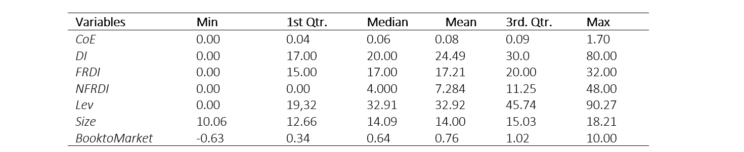
Note: CoE is the estimation of the cost of equity calculated according to (3); DI, the risk disclosure index calculated according to (4); FRDI, the financial risk disclosure index calculated according to (5); NFRDI, the non-financial risk disclosure index calculated according to (6); Lev, the ratio of total debt to market capitalization; Size, the logarithm of market capitalization; and BooktoMarket, the book-to-market ratio.
4. RESULTS
Table 2 presents the results of the regression analysis, based on the Bayesian methodology, and the estimates obtained for the two proposed models. The first model includes disclosed risk information as a whole, while the second one differentiates information related to financial risks and information related to non-financial risks.
The estimated coefficients based on the Bayesian analysis cannot be interpreted in the same terms as the classical statistical analysis. It is true that the coefficient value of each variable provided by the Bayesian approach (which corresponds to the average value of the posterior probability distribution for that coefficient) coincides with the value of the coefficients obtained by a conventional regression analysis (e.g., ordinary least squares). As a matter of fact, one may interpret the parameters of the “MEAN” column in Table 2 in the same way as those of the coefficients of a classical regression model. For example, the positive value (0.0009) of the variable Lev in Model 1 (see Table 2) tells us how much the cost of equity (dependent variable) will increase in case of a unitary change in Lev.
Tabla 2. Resumen de la distribución a posteriori de los Modelos 1 y 2
| Model 1 | Model 2 | ||||||
| MEAN | SD | P(β > 0)% | MEAN | SD | P(β > 0)% | ||
| (Intercept) | -0.1530 | 0.0407 | 3.00 | -0.1774 | 0.0439 | 1.00 | |
| DI | 0.0002 | 0.0004 | 72.22 | ||||
| FRDI | 0.0020 | 0.0012 | 95.35 | ||||
| NFRDI | -0.0003 | 0.0005 | 28.28 | ||||
| Lev | 0.0009 | 0.0002 | 99.98 | 0.0008 | 0.0002 | 99.92 | |
| Size | 0.0093 | 0.0028 | 99.96 | 0.0093 | 0.0028 | 99.93 | |
| BooktoMarket | 0.0864 | 0.0065 | >99.99 | 0.0879 | 0.0066 | >99.99 | |
| sigma2 | 0.0077 | 0.0005 | 99.99 | 0.0077 | 0.0005 | 99.99 | |
Note: CoE is the estimation of the cost of equity calculated according to (3); DI, the risk disclosure index calculated according to (4); FRDI, the financial risk disclosure index calculated according to (5); NFRDI, the non-financial risk disclosure index calculated according to (6); Lev, the ratio of total debt to market capitalization; Size, the logarithm of market capitalization; and BooktoMarket, the book-to-market ratio.
However, when we carry out the classical analysis, the only inference we can draw from the coefficient’s value is to establish whether or not it is significantly equal to (or higher than) a certain value (usually 0). The Bayesian analysis, as described above, allows us to determine a degree of probability, i.e., we can assess the probability of the estimated coefficient being equal to (or higher than) a certain value.
For example, in the case of the variable Size in Model 1, the average value of the coefficient’s posterior distribution (which coincides with the estimated value in a classical regression model) is 0.0093. The probability of this coefficient being higher than 0 is 99.96 % (see Table 2). We were able to calculate this last value because of the Bayesian analysis, which allows us to establish the statistical distribution of the coefficient. Thus, we obtained not only a point estimate, but also its density function. Similarly, we can apply this logic to the rest of the control variables of the two estimated models (see Figure 1).
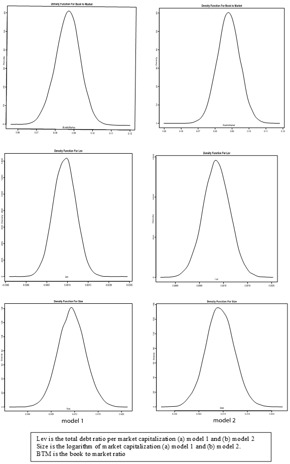
Figura 1. Función de densidad a posteriori de las variables de control (Modelos 1 y 2)
Source: Own elaboration with research results.
Regarding the risk information disclosed by firms, Table 2 shows that
the coefficient of the variable that refers to disclosed information as a whole
(DI) presents an average value of 0.0002 (the 95% credible intervals for the
variables can be seen in tables 3 and 4). Beyond this relatively low average
value, the most relevant number is the probability that this coefficient is
higher than zero: 72.22 % (Figure 2 shows the density function of the
parameter’s posterior distribution). Consequently, since there is a high
probability (27.78 %) that the parameter is less than 0, it would be risky (in
terms of probability) to make a prediction about its sign. In short, we cannot
conclude anything about the sign of this coefficient. Therefore, the variable
will probably be irrelevant in the estimated model. This means that, when a
company discloses risk information as a whole, it does not influence the cost
of equity. These results contradict the theoretical assumptions of
Tabla 3. Intervalos de credibilidad al 95% para las variables del modelo 1

Note: DI is the risk disclosure index calculated according to (4); Lev is the ratio of total debt to market capitalization; Size is the logarithm of market capitalization; BooktoMarket is the book-to-market ratio.
Tabla 4. Intervalos de credibilidad al 95% para las variables del modelo 2

Note: FRDI is the financial risk disclosure index calculated according to (5); NFRDI is the non-financial risk disclosure index calculated according to (6); Lev is the ratio of total debt to market capitalization; Size is the logarithm of market capitalization; BooktoMarket is the book-to-market ratio.
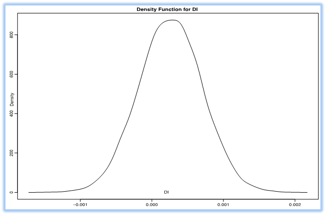
Fig. 2. Posterior density of DI (Model 1)
Figura 2. Función de densidad a posteriori de DI (Modelo 1)
Source: Created by the authors.
Model 2 differentiates between financial and non-financial risk information. Additionally, the average values of the estimated coefficients are 0.0020 and 0.0003 for FRDI and NFRDI, respectively. As can be seen from Table 2, the probability of the coefficient of the latter (regarding information on non-financial risks) being higher than 0 is 28.28%, i.e., we cannot categorically state that its coefficient’s sign is negative since there is also a high probability of it being positive (see Figure 3). Consequently, these results lead us to conclude that the information disclosed about non-financial risks does not influence the cost of equity.
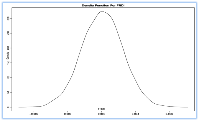
Figure 3. Posterior density of FRDI (Model 2)
Figura 3. Función de densidad a posteriori de FRDI (Modelo 2)
Source: Created by the authors.
However, the situation for FRDI is different: the
probability that the value of the coefficient of this variable is positive is
95.35% (see Table 2). Based on this level of probability, we can say that this
coefficient is higher than 0 (also see Figure 4). Consequently, it can be
pointed out that financial risk disclosure is related to cost of equity. A
higher degree of financial risk disclosure is perceived by investors as a
greater risk factor and thus requires higher costs. These results concur well
with the theoretical assumptions of
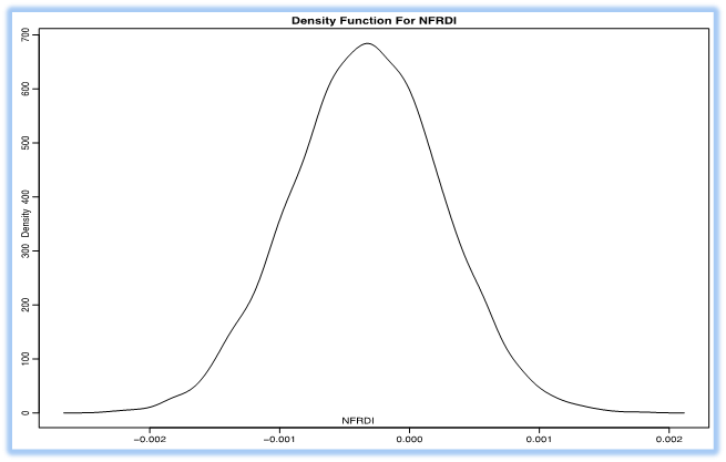
Figure 4. Posterior density of NFRDI (Model 2)
Figura 4. Función de densidad a posteriori de NFRDI (Modelo 2)
Source: Created by the authors.
5. CONCLUSIONS
There is abundant literature on the relationship between the information published by corporations and their cost of equity. However, in said literature, few studies have addressed the relationship between cost of equity and corporate risk disclosure. Our study focused on this subject and made an additional contribution in terms of the methodology we adopted: A Bayesian analysis using the Markov Chain Monte Carlo Method (MCMC). In effect, to date, all the studies that have empirically analyzed the relationship between disclosed information and cost of equity have applied a classical statistical approach, which only allows us to establish whether there is a significant relationship between cost of equity and the information variables under study. In other words, the classical analysis only enables us to infer a yes/no type of relationship among variables. The Bayesian analysis, however, allows us to go one step further and assign probabilities to the estimates of the model’s parameters.
We applied this methodology to a sample of firms listed on the Spanish Stock Market. Our results show that the cost of equity and disclosed risk information (when a global view of the later is adopted) are not related. However, when risk information is divided into financial and non-financial risks, a significant relationship can be found. Specifically, there is a relationship between cost of equity and the financial risk information disclosed by firms. The positive sign of this relationship indicates that, for the market, greater risk information means a greater level of risk, which involves a higher cost of equity for the company.
NOTAS AL PIE
- arrow_upward 1 We initialize the algorithm with random values. Therefore, the samples simulated based on this algorithm, at early iterations, may not necessarily be representative of the actual posterior distribution. These samples are commonly discarded. The discarded iterations are often referred to as the “burn-in” period.
- arrow_upward 2 Strictly speaking, MCMC methods do not provide us with the posterior density function, only random samples from it. The posterior distribution can then be built from the moments of these samples.
- arrow_upward * This article is derived from the project entitled "Risk Disclosure and Cost of Equity: A Bayesian Approach" and has been financed with own resources.
REFERENCES
- arrow_upward Abraham, S. & Cox, P. (2007). Analysing the determinants of narrative risk information in UK FTSE 100 annual reports. The Bristish Accounting Review, 39(3), 227-248. https://doi.org/10.1016/j.bar.2007.06.002
- arrow_upward Alamilla-López, N. E., & Jiménez, J. C. (2010). Contraste de Hipótesis: Clásico vs. Bayesiano. Revista Digital Matemática Educación e Internet, 11(1), 1-13. https://tecdigital.tec.ac.cr/revistamatematica/ARTICULOS_V11_N1_2010/NAlamilla_ConstrastedeHipotesis/index.html
- arrow_upward Albarrak, M. S., Elnahass, M., Papagiannidis, S., & Salama, A. (2020). The effect of twitter dissemination on cost of equity: A big data approach. International Journal of Information Management, 50, 1-16. https://doi.org/10.1016/j.ijinfomgt.2019.04.014
- arrow_upward Beyer, A., Cohen, D. A., Lys, T. Z., & Walther, B. R. (2010). The Financial Reporting Environment: Review of the Recent Literature. Journal of Accounting and Economics, 50(2-3), 296-343. https://doi.org/10.1016/j.jacceco.2010.10.003
- arrow_upward Blanco, B., Garcia Lara, J. M., & Tribo, J. A. (2015). Segment Disclosure and Cost of Capital. Journal of Business Finance & Accounting, 42(3-4), 367-411. https://doi.org/10.1111/jbfa.12106
- arrow_upward Botosan, C. A. (1997). Disclosure Level and the Cost of Equity Capital. The Accounting Review, 72(3), 323-349. https://www.jstor.org/stable/248475
- arrow_upward Botosan, C. A., & Plumlee, M. A. (2002). A Re-examination of Disclosure Level and Expected Cost of Equity Capital. Journal of Accounting Research, 40(1), 21-40. http://dx.doi.org/10.1111/1475-679X.00037
- arrow_upward Botosan, C. A., & Plumlee, M. (2005). Assessing Alternative Proxies for the Expected Risk Premium. The Accounting Review, 80(1), 21-53. https://doi.org/10.2308/accr.2005.80.1.21
- arrow_upward Cabedo, J. D., & Tirado, J. M. (2004). The disclosure of risk in financial statements. Accounting Forum, 28(2), 181-200. https://doi.org/10.1016/j.accfor.2003.10.002
- arrow_upward Campbell, J. L., Chen, H., Dhaliwal, D. S., Lu, H. M., & Steele, L. B. (2014). The information content of mandatory risk factor disclosures in corporate filings. Review of Accounting Studies, 19(1), 396-455. https://doi.org/10.1007/s11142-013-9258-3
- arrow_upward Campbell, J. L., Chen, H., Dhaliwal, D. S., Lu, H. M., & Steele, L. B. (2014). The information content of mandatory risk factor disclosures in corporate filings. Review of Accounting Studies, 19(1), 396-455. https://doi.org/10.1007/s11142-013-9258-3
- arrow_upward Cheng, F., Jorgensen, B. N., & Yoo, Y. K. (2004). Implied cost of equity capital in earnings-based valuation: International evidence. Accounting and Business Research, 34(4), 323-344. https://doi.org/10.1080/00014788.2004.9729975
- arrow_upward Clarkson, P., Guedes, J., & Thompson, R. (1996). On the diversification, observability, and measurement of estimation risk. Journal of Financial and Quantitative Analysis, 31(1), 69-84. https://doi.org/10.2307/2331387
- arrow_upward Diamond, D. W., & Verrecchia, R. E. (1991). Disclosure, Liquidity, and the Cost of Capital. Journal of Finance, 46(4), 1325-1359. https://doi.org/10.1111/j.1540-6261.1991.tb04620.x
- arrow_upward Easley, D., & O'hara, M. (2004). Information and the Cost of Capital. The Journal of Finance, 59(4), 1553-1583. https://doi.org/10.1111/j.1540-6261.2004.00672.x
- arrow_upward Easton, P. D. (2004). PE ratios, PEG Ratios, and Estimating the Implied Expected Rate of Return on Equity Capital. The Accounting Review, 79(1), 73-95. http://dx.doi.org/10.2139/ssrn.423601
- arrow_upward Embong, Z., Mond-Saleh, N., & Hassan, M. S. (2012). Firm Size, Disclosure and Cost of Equity Capital. Asian Review of Accounting, 20(2), 119-139. https://doi.org/10.1108/13217341211242178
- arrow_upward Filzen, J. J. (2015). The Information Content of Risk Factor Disclosures in Quarterly Reports. Accounting Horizons, 29(4), 887-916. https://doi.org/10.2308/acch-51175
- arrow_upward Francis, J. R., Khurana, I. K., & Pereira, R. (2005). Disclosure incentives and effects on cost of capital around the world. The Accounting Review, 80(4), 1125-1162. https://doi.org/10.2308/accr.2005.80.4.1125
- arrow_upward Francis, J., Nanda, D., & Olsson, P. (2008). Voluntary Disclosure, Earnings Quality, and Cost of Capital. Journal of Accounting Research, 46(1), 53-99. https://doi.org/10.1111/j.1475-679X.2008.00267.x
- arrow_upward Gebhardt, W. R., Lee, C. M. C., & Swaminathan, B. (2001). Toward an Implied Cost of Capital. Journal of Accounting Research, 39(1), 135-176. https://doi.org/10.1111/1475-679X.00007
- arrow_upward Gietzmann, M., & Ireland, J. (2005). Cost of Capital, Strategic Disclosures and Accounting Choice. Journal of Business Finance & Accounting, 32(3-4), 599-634. https://doi.org/10.1111/j.0306-686X.2005.00606.x
- arrow_upward Gietzmann, M. B., & Trombetta, M. (2003). Disclosure interactions: accounting policy choice and voluntary disclosure effects on the cost of raising outside capital. Accounting and Business Research, 33(3), 187-205. https://doi.org/10.1080/00014788.2003.9729646
- arrow_upward Gilks, W. R., Richardson, S., & Spiegelhalter, D. J. (Eds.). (1996). Markov Chain Monte Carlo in Practice. Chapman & Hall.
- arrow_upward Hahn, E. D. (2014). Bayesian Methods for Management and Business: Pragmatic Solutions for Real Problems. John Wiley & Sons.
- arrow_upward Hail, L. (2002). The Impact of Voluntary Corporate Disclosures on the Ex Ante Cost of Capital for Swiss Firms. European Accounting Review, 11(4), 741-773. http://dx.doi.org/10.2139/ssrn.279276
- arrow_upwardHail, L. & Leuz, C. L. (2006). International Differences in the Cost of Equity Capital: Do Legal Institutions and Securities Regulation Matter? Journal of Accounting Research, 44(3), 485-531. https://doi.org/10.1111/j.1475-679X.2006.00209.x
- arrow_upward Heinle, M. S., & Smith, K. C. (2017). A theory of risk disclosure. Review of Accounting Studies, 22(4), 1459-1491. https://doi.org/10.1007/s11142-017-9414-2
- arrow_upwardHope, O. K., Hu, D., & Lu, H. (2016). The benefits of specific risk-factor disclosures. Review of Accounting Studies, 21(4), 1005-1045. https://doi.org/10.1007/s11142-016-9371-1
- arrow_upward Jorgensen, B. N., & Kirschenheiter, M. T. (2003). Discretionary Risk Disclosures. The Accounting Review, 78(2), 449-469. https://doi.org/10.2308/accr.2003.78.2.449
- arrow_upward Jorgensen, B. N., & Kirschenheiter, M. T. (2003). Discretionary Risk Disclosures. The Accounting Review, 78(2), 449-469. https://doi.org/10.2308/accr.2003.78.2.449
- arrow_upward Jorgensen, B. N., & Kirschenheiter, M. T. (2003). Discretionary Risk Disclosures. The Accounting Review, 78(2), 449-469. https://doi.org/10.2308/accr.2003.78.2.449
- arrow_upward Jorion, P. (2002). How Informative Are Value‐at‐Risk Disclosures? The Accounting Review, 77(4), 911-931. https://doi.org/10.2308/accr.2002.77.4.911
- arrow_upward Kim, O., & Verrecchia, R. E. (1994). Market liquidity and volume around earnings announcements. Journal of Accounting and Economics, 17(1-2), 41-67. https://doi.org/10.1016/0165-4101(94)90004-3
- arrow_upwardKothari, S. P., Li, X., & Short, J. E. (2009). The Effect of Disclosures by Management, Analysts, and Business Press on Cost of Capital, Return Volatility, and Analyst Forecasts: A Study Using Content Analysis. The Accounting Review, 84(5), 1639-1670. https://doi.org/10.2308/accr.2009.84.5.1639
- arrow_upward Kravet, T., & Muslu, V. (2013). Textual risk disclosures and investors’ risk perceptions. Review of Accounting Studies, 18,1088-1122. https://doi.org/10.1007/s11142-013-9228-9
- arrow_upward Lan, Y., Wang, L., & Zhang, X. (2013). Determinants and features of voluntary disclosure in the Chinese stock Market. China Journal of Accounting Research, 6(4), 265-285. https://doi.org/10.1016/j.cjar.2013.04.001
- arrow_upward Leuz, C., & Verrecchia, R. E. (2000). The Economic Consequences of Increased Disclosure. Journal of Accounting Research, 38, 91-124. http://dx.doi.org/10.2139/ssrn.171975
- arrow_upward Linsley, P. M., & Shrives, P. J. (2006). Risk Reporting: A study of risk disclosures in the annual reports of UK companies. The British Accounting Review, 38(4), 387-404. https://doi.org/10.1016/j.bar.2006.05.002
- arrow_upward Martin, A. D., Quinn, K. M., & Park, J. H. (2011). MCMCpack: Markov Chain Monte Carlo in R. Journal of Statistical Software, 42(9), 1-21. https://doi.org/10.18637/jss.v042.i09
- arrow_upward Miihkinen, A. (2013). The usefulness of firm risk disclosures under different firm riskiness, investor-interest, and market conditions: New evidence from Finland. Advances in Accounting, 29(2), 312-331. https://doi.org/10.1016/j.adiac.2013.09.006
- arrow_upward Mohobbot, A. M. (2005). Corporate risk reporting practices in annual reports of Japanese companies. http://jaias.org/2005bulletin/p113Ali%20Md.Mohobbot.pdf
- arrow_upward Nahar, S., Azim, M., & Anne Jubb, C. (2016). Risk disclosure, cost of capital and bank performance. International Journal of Accounting & Information Management, 24(4), 476-494. https://doi.org/10.1108/IJAIM-02-2016-0016
- arrow_upward Nelson, M. W. and Rupar, K. K. (2015). Numerical Formats within Risk Disclosures and the Moderating Effect of Investors' Concerns about Management Discretion. The Accounting Review, 90(3), 1149-1168. https://doi.org/10.2308/accr-50916
- arrow_upward Peasnell, K. V. (1997). Financial Reporting of Risk: Proposals for a Statement of Business Risk. Institute of Chartered Accountants in England and Wales.
- arrow_upward Rajgopal, S. (1999). Early Evidence on the Informativeness of the SEC's Market Risk Disclosures: The Case of Commodity Price Risk Exposure of Oil and Gas Producers. The Accounting Review, 74(3), 251-280. https://doi.org/10.2308/accr.1999.74.3.251
- arrow_upward Richardson, A. J., & Welker, M. (2001). Social disclosures, financial disclosure and the cost of equity capital.Accounting, Organizations and Society, 26(7-8), 597-616. https://doi.org/10.1016/S0361-3682(01)00025-3
- arrow_upward Solomon, J. F., Solomon, A., Norton, S. D., & Joseph, N. L. (2000). A conceptual framework for corporate risk disclosure emerging from the agenda for corporate governance reform. The British Accounting Review, 32(4), 447-478. https://doi.org/10.1006/bare.2000.0145
- arrow_upward Verrecchia, R. E. (1999). Disclosure and the cost of capital: A discussion. Journal of Accounting and Economics, 26(1-3), 271-283. https://doi.org/10.1016/S0165-4101(98)00041-X
- arrow_upward Zellner, A. (1996). An Introduction to Bayesian Inference in Econometrics. John Wiley & Sons.