Cournot-Nash Equilibrium and Perfect Competition in the Solow-Uzawa Growth Model*
Equilibrio de Cournot-Nash y competencia perfecta en el modelo de crecimiento de Solow-Uzawa
Received: 2 march 2021
Accepted: 1 june 2021
Abstract
The purpose of this study is to contribute to economic growth theory by introducing Cournot competition into the Solow-Uzawa neoclassical growth model with Zhang’s concept of disposable income and utility function. The Solow-Uzawa two-sector growth model deals with economic growth with two sectors with all the markets perfectly competitive. The final goods sector in this study is the same as that in the Solow model with perfect competition. The consumer goods sector is composed of two firms and characterized by Cournot competition. All the input factors are traded in perfectly competitive markets. The duopoly’s product is solely consumed by consumers. Perfectly competitive firms earn zero profit, while duopolists earn positive profits. This study assumes that the population shares the profits equally. First, we built the dynamic model. Afterward, we found a computational procedure to describe the time-dependent path of the economy and conducted comparative dynamic analyses of some parameters. Finally, we compared the economic performances of the model with Cournot competition and the perfectly competitive model.
Keywords: Cournot game, perfect competition, Nash equilibrium, Solow model, Uzawa model.
JEL Classification: F12, F43, N30.
Highlights
Resumen
El propósito de este estudio es contribuir a la teoría del crecimiento económico por medio de la introducción de la competencia de Cournot en el modelo neoclásico del crecimiento económico de Solow-Uzawa con el concepto de ingreso disponible y la función de utilidad de Zhang. El modelo de crecimiento de dos sectores de Solow-Uzawa maneja el crecimiento económico con dos sectores con todos los mercados perfectamente competitivos. En este trabajo, el sector de bienes finales es el mismo que en el modelo de Solow con competencia perfecta. El sector de bienes de consumo está compuesto por dos firmas y se caracteriza por la competencia de Cournot. Todos los factores de entrada se intercambian en mercados perfectamente competitivos. Solo los consumidores consumen el producto del duopolio. Las firmas perfectamente competitivas tienen una ganancia igual a cero, mientras que las duopolistas tienen ganancias positivas. En este estudio se asume que la población comparte las ganancias de forma equitativa. Primero, construimos un modelo dinámico. Después, encontramos un procedimiento computacional para describir el movimiento de la economía dependiendo del tiempo y realizamos análisis dinámicos comparativos de algunos parámetros. Finalmente, comparamos los desempeños económicos del modelo con competencia de Cournot y el modelo perfectamente competitivo.
Palabras clave: juego de Cournot, competencia perfecta, equilibrio de Nash, modelo de Solow, modelo de Uzawa.
Clasificación JEL: F12, F43, N30.
Highlights
1. INTRODUCTION
The objective of this paper is to introduce imperfect competition (Cournot game) of market structure, which has been well examined in industrial economics, into neoclassical growth theory with an alternative approach to the saving behavior of households. Neoclassical growth theory is especially concerned with the interdependence between wealth accumulation and production under simplified market structures (
Cournot (1801–1877) proposed the theory of Cournot competition in 1838 when he examined a market dominated by duopoly. He constructed profit and best response functions for each firm for a given exogenous output level of the other firm. An equilibrium is identified where these best response functions intersect. The Cournot model has now become a standard model to analyze market structure in microeconomics. This study introduces the aforementioned market structure into neoclassical growth theory with wealth/capital accumulation. We considered an industrial market characterized by Cournot duopoly that supplies a homogenous product. Price is a known function of total output of each duopolist. Each duopolist takes the output of the other as given when it maximizes its profit. Each duopolist’s cost function is assumed to be common knowledge. The cost functions and production functions of each firm are different. The market price is determined when the demand is equal to the total quantity supplied by the duopoly. Each duopolist considers the quantity supplied by the other as given, evaluates its residual demand, and then behaves as a monopoly.
The macro framework of this study is founded on the Solow-Uzawa neoclassical model. The mechanism of economic growth is wealth accumulation. Most formal models in the literature of neoclassical growth economic theory with endogenous wealth accumulation are developed for economies with perfectly competitive markets (
The rest of this paper is organized as follows: In Section 2, we build a growth model of perfect and Cournot competition with endogenous wealth accumulation. In Section 3, we study analytical properties of the economic system and identify the existence of a point of equilibrium. In Section 4, we carry out a comparative static analysis of a few parameters. Finally, in Section 5, we draw the conclusions of this study.
2. THEORETICAL FRAMEWORK
The two-sector growth model with perfect and Cournot competition
This study integrates Cournot competition into the Solow-Uzawa neoclassical growth model with Zhang’s concept of disposable income and utility function. For the sake of simplicity, we deal with a duopoly here. The model can be generalized in a straightforward manner in case of any number of firms in Cournot competition. Most aspects of the model are basically the same as those in the Solow-Uzawa two-sector growth model, except for the modelling of household behavior and duopoly behavior. The economy supplies final goods and products of the duopoly. The final goods sector is perfectly competitive and produces capital goods as in the Solow model. Capital goods are invested and consumed. The final goods sector is the same as the one in the Solow model. We follow the Uzawa two-sector model regarding the modelling of the economic structure. In the Uzawa model, it is assumed that the consumer goods sector is composed of two firms and characterized by Cournot competition. In our model, all input factors are supplied competitively. The duopoly’s product is solely consumed by consumers. The final goods sector and duopolists use capital and labor as inputs to produce final goods and duopoly’s products. In perfect markets (homogenous), firms have zero profit, while a duopoly might have positive profits. This study assumes that the homogeneous population shares profits equally. There is no free entry in a duopoly market. In addition, the final good is expressed in numeraire, which serves as a medium of exchange. It is assumed that capital depreciates at a fixed depreciation rate of δk
Production of final products
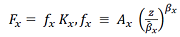
Let Fi (t), Ki (t), and Ni (t) stand for output, capital input, and labor inputs of the final goods sector, respectively. The production function of the final goods sector is specified as follows (1):
Where Ai, ai and βi are parameters. We use w(t) and r(t) to denote the wage and interest rates, respectively. The input prices are equal for all the producers due to perfect competition in input factors markets. The profit of the final goods sector is
The marginal conditions imply (2):
Where
`r_δ (t)≡r(t)+δ_k`
Consumer behaviors and wealth dynamics
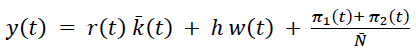
This study applies the approach to modeling household behavior proposed by Zhang (1993, 2005). We use k ̄ (t) to denote wealth per household. In addition, we have k ̄ (t) = K(t) / N ̄ , where K(t) is the total capital. It is assumed that profits, due to the duopoly, are equally shared among the population. Note that profits, in the literature of industrial economics, are often assumed to be invested in innovation. Conceptually, it is not difficult to make profit distribution more realistic by including endogenous technologies. Here, we use to represent human capital and πj (t) to denote duopolist j's profit. The current income of the representative household is obtained as follows (3):
 (3)
(3)
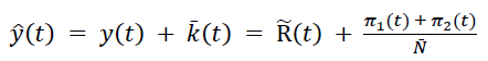
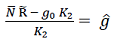
The household’s disposable income, i.e., y ̂ (t), equals the current disposable income and the value of wealth as follows (4):
 (4)
(4)
where
The representative household distributes the total available budget among the consumption of the duopoly’s product cs(t), the consumption of final goods ci(t), and savings s(t). The budget constraint is (5):
where p(t) is the price of the duopoly’s product It is assumed that the U(t) utility level is related to cs(t), ci(t), and s(t) as follows:
`U(t)=c_s^(η_0 ) (t) c_i^(ξ_0 ) (t) s^(λ_0 ) (t),η_0,ξ_0,λ_0 > 0`
where λ0 denotes the propensity to save. We solve the optimal problem (6):
Where
There is a proportional relationship between the disposable income and the total value of the variable. This simple relationship is due to the presumed utility functional form. We conclude that, once we determine p(t) and y ̂ (t), we can determine the behavior of the household.
Wealth accumulation
According to the definition of s(t), the change in the representative household’s wealth is calculated as follows (7):
According to this equation, the change in wealth equals saving minus dissaving.
Equilibrium for the duopoly’s product
We denote the output of duopolist j using Fj (t) The equilibrium condition for the duopoly’s product is (8):
Duopoly behavior
Duopolies are characterized by Cournot competition. Companies in the consumer goods industry compete over the amount of output they will supply. Each firm decides independently of other firms at the same time. They do not cooperate and compete in quantities. They choose quantities simultaneously. There is no product differentiation between the firms. Firms have market power as each firm’s output decision influences the price of the duopoly’s goods. They behave economically rationally, and each firm designs its strategies with the aim of maximizing profit given the other firm’s decisions on quantities.
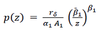
From (8) and (6), the demand function for the duopoly’s product is given by (9):
Where Fd(t) ≡ F1(t) + F2(t). We use Kj(t) and Nj(t) to represent duopolist j’s capital input and labor input, respectively. The production functions of the duopoly are taken on the following form (10):
Where Aj, aj, and βj are parameters. The profit of duopolist j is given by (11):
Inserting (9) in (11), we get (12):
Adding the two equations in (12) yields (13):
where
Inserting (13) in (12), we obtain (14):
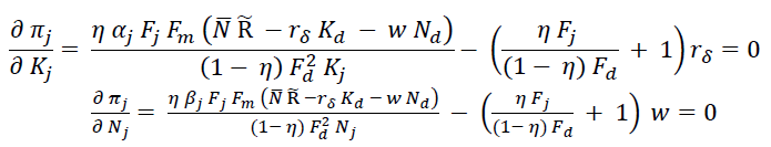
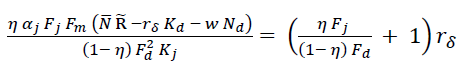
Each duopolist maximizes its profit given the other duopolist’s output (and input factors). The marginal conditions are the following (15):
 (15)
(15)
According to (15), each duopolist decides on the labor and capital inputs as functions of the wage rate, interest rate, wealth, and the other duopolist’s output and input factors. Each duopolist’s output and profit are determined by (10) and (14), respectively. The price of the duopoly’s product is given by (9).
Demand and supply of final goods
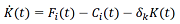
The change in capital stock equals the output of the final goods sector minus the depreciation of the capital stock and total consumption. The physical capital accumulation equation is given as follows (16):
 (16)
(16)
where
Labor and capital being fully utilized
In an equilibrium of the labor market, we have (17):
For capital markets, we have (18):
 (18)
(18)
We have thus constructed the model proposed here, which is founded on the Solow-Uzawa model (
3. METHOD
In the previous section, we constructed the growth model of wealth accumulation with perfect competition and Cournot game. The following lemma presents a computational program to follow the movement of the economic system. We thus introduce a variable:
LemmaThe dynamics of the economic system are described by the following differential equation (19):
where φ ̅ (z(t)) is the function of z(t) defined in the Appendix. All the other variables are explicitly given as functions of z(t), as follows: K ̅ (t) by (A15) → K(t) =k ̄ (t) N ̄ → r(t) by (A2) → w(t) by (A3) → K2(t) by (A12) → K1(t) by (A10) → Ki(t) by (A11) → N1(t), N2(t) and Ni(t) by (A1) →Fi(t) and Fj(t) by (A4) → R ̄ (t) by (4) → πj(t) by (14) → y ̂ (t) by (4) → p(t) by (9) → ci(t), cs(t) and s(t) by (7) → U(t) by the definition.
To simulate the model, we specified the values of the parameters as follows (20)
 (20)
(20)The population is 50, and the human capital is 2. The selected values of the parameters do not refer to a real-life economy. We gain insight into the economic mechanism of growth by simulating the effects of different values of these parameters on the national economy. We defined the following initial condition: z (0) = 0.102. The movement is given by Figure 1, where the growth rate is defined by (21):
 (21)
(21)
Where
`Y(t)= F_i (t)+ p(t) F_d (t)`
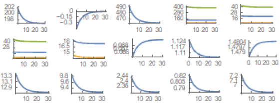
Figura 1. Movimiento del sistema económico
Source: Created by the author.
From the initial state, the national output falls. The growth rate is negative and is zero in equilibrium. The profits of duopolists fall. The three levels of output of the sectors change slightly. The profit of the duopoly’s product increases, and the interest rate rises. The wage rate falls. The representative household has a lower income, consumes less, and has a lower utility. The simulation demonstrates that the system becomes stationary in the long term. The simulation gives the equilibrium point as follows:
The eigenvalue at the point of equilibrium is – 0.183. This implies that the point of equilibrium is locally stable and that the dynamic comparative analysis is effective in the transitory process as well as in the long term.
4. RESULTS AND DISCUSSION
In the previous section, we demonstrated the movement of the national economy with perfectly competitive and duopoly product markets. This section examines how the national economic movement is affected when some exogenous conditions, such as households’ preference and technologies, experience exogeneous changes. Following the computational procedure to calibrate the model in the lemma, we describe the effects of changes in any parameter on the movement of the economic system. Let us define a variable Δ ̄x to denote the change rate of the x variable in percentage due to changes in the parameter value.
Duopolist 1’s total factor productivity is enhanced
We first examine how the national economy changes its path of development when one duopolist’s total factor productivity is enhanced as follows: Δ ̄A1 = 3.3. The effects of this modification on the variables are plotted in Figure 2. The output of duopolist 1 is increased. Duopolist 1 employs less labor and capital inputs. Duopolist 2 produces less and employs less labor and capital inputs. Duopolist 1 gets more profit, while duopolist 2 gets less of it. The final goods sector produces more and employs more labor and capital inputs. The growth rate is enhanced. The national output is augmented. The interest rate falls. The wage rate rises. The price of the duopoly’s product is reduced. The representative household has more wealth and disposable income. The utility is enhanced. The household consumes more final goods and duopoly’s product.
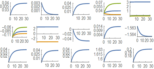
Figura 2. La productividad total de los factores del duopolista 1 mejora
Source: Created by the author.
The propensity to consume the duopoly’s product is augmented
We now study how the national economy is affected when the propensity to consume the duopoly’s product is augmented as follows: Δ ̄ η0 = 10. The effects on the variables are plotted in Figure 3. The output levels of the two duopolists are increased. Each duopolist employs more labor and capital inputs. Their profits are enhanced. The final goods sector produces less and employs less labor and capital inputs. The growth rate is reduced. The national output is augmented. The interest rate rises, and the wage rate falls. The price of the duopoly’s product is enhanced. The utility is enhanced initially but reduced in the long term. The household has less wealth and disposable income. The household consumes fewer final goods but more duopoly’s product.
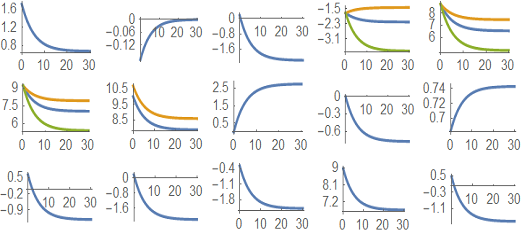
Figura 3. Se aumenta la propensión a consumir el producto del duopolio
Source: Created by the author.
The propensity to save is augmented
We now study how the movement of the national economy changes when the propensity to save is enhanced as follows: Δ ̄ λ0 = 1.15. The effects on the variables are plotted in Figure 4. The national physical capital is increased. The national output falls initially but rises in the long term. The output levels of the two duopolists are reduced initially but increased in the long term. Each duopolist employs less capital input initially but more of it in the long term. Each duopolist employs less labor input. Their profits are reduced initially but enhanced in the long term. The final goods sector produces more and employs more labor and capital inputs. The growth rate is enhanced. The interest rate falls, and the wage rate rises. The price of the duopoly’s product is reduced. The utility is enhanced. The household has more wealth and disposable income. The household consumes fewer final goods and duopoly’s product initially but more final goods and duopoly’s product in the long term.

Figura 4. La propensión a ahorrar aumenta
Source: Created by the author.
The final goods sector’s total factor productivity is enhanced
We now study how the national economy is affected when the propensity to consume the duopoly’s product is augmented as follows: Δ ̄ Ai = 5. The effects on the variables are plotted in Figure 5. The final goods sector produces more and employs more capital input. The sector employs more labor force initially but does not change labor input in the long term. The output levels of the two duopolists are reduced initially but increased in the long term. Each duopolist employs less capital input initially but more of it in the long term. It employs less labor input initially but it does not change in the long term. Their profits are enhanced. The growth rate is augmented. The national output is augmented. The interest rate rises initially but does not change in the long term. The wage rate rises. The price of the duopoly’s product is enhanced. The household has more wealth and disposable income. The utility is enhanced. The household consumes more final goods. The household consumes less duopoly’s product initially but more of it in the long term.
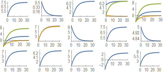
Figura 5. La productividad total de los factores del sector de bienes finales mejora
Source: Created by the author.
Duopolist 1’s output elasticity of capital input is augmented
We now analyze how the national economy is affected when duopolist 1’s output elasticity of capital input is augmented as follows: Δ ̄ ai = 10. The effects on the variables are plotted in Figure 6. The national capital stock and national output rise initially and do not change in the long term. The output level of duopolist 1 is enhanced. Duopolist 1 produces and employs more capital input and less labor input. Duopolist 2 produces more initially but produces the same amount in the long term. It employs more capital input initially and less of it in the long term. It uses more labor input. Duopolist 1 has more profit, while duopolist 2 has less profit. The final goods sector produces more initially and almost the same amount in the long term. Said sector uses more labor input. It employs more capital input initially and less of it in the long term. The interest rate rises, and the wage rate falls. The price of the duopoly’s product is reduced. The utility is enhanced initially but changed slightly in the long term. The household has more wealth and disposable income initially but almost the same amount in the long term. The household consumes more final goods initially but almost the same number in the long term. The household consumes more duopoly’s product.
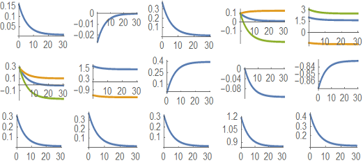
Figura 6. La elasticidad de salida de la entrada de capital del duopolista 1 se incrementa
Source: Created by the author.
Comparison with perfect competition
This section compares the dynamics of the model proposed with Cournot competition and the two-sector model with perfect competition. When the system is perfectly competitive, firms take the price as given, and the equilibrium condition of demand and supply determines the price. We here describe the growth model when the consumer goods market is perfectly competitive. One of the main differences is that the profit is zero in perfect competition, i.e., πj (t)=0. The profits and marginal conditions for the two firms are the following, respectively:
where Equations (11)’ and (15)’ correspond to (11) and (15), respectively. The rest of the equations in Section 2, except those related to the duopoly’s profits and marginal conditions, hold as well for the perfectly competitive case. In Appendix A-2, we present a computational program to plot the movement of the competitive model. We plot the movement of the two systems under the same parameter values in (20). The result is plotted in Figure 7. In the latter, we do not plot profits as no firm achieves a positive profit in the perfectly competitive economy. In our model, firm 2 produces nothing in the case of the perfectly competitive economy. Hence, firm 1’s behavior represents the sector’s behavior. From the figure, we conclude that, in the Cournot competition, the national output and national capital (and thus household wealth) are higher than in the perfectly competitive economy. In the Cournot competition, the final goods sector produces more and employs more labor and capital inputs, while the consumer goods sector produces less and employs less labor and capital inputs. The interest rate is lower, the wage rate is higher, and the price of consumer goods is higher. The household has more disposable income, consumes more final goods, consumes fewer consumer goods, and has a higher level of utility. We see that, if the profits of the duopoly are equally distributed among the households, the welfare of the latter is higher welfare when the consumer goods market is characterized by Cournot competition rather than perfect competition.
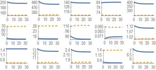
Figura 7. Comparación del movimiento de los dos sistemas económicos
Source: Created by the author.
5. CONCLUSIONS
This study made a unique contribution to economic growth theory by integrating an important model of industry structure with imperfect competition in microeconomic theory with neoclassical growth theory. The proposed model shows a way to integrate neoclassical economic growth theory with modern microeconomics. We introduced Cournot competition into the Solow-Uzawa neoclassical growth model with Zhang’s concept of disposable income and utility function. The model is founded on some well-known economic theories in economic literature. The economy analyzed here is composed of final goods and consumer goods sectors. We constructed the model within the framework of the Solow-Uzawa two-sector growth model. The final goods sector is the same as that in the Solow model, in which all markets are perfectly competitive. We followed the Uzawa’s two-sector model of economic growth but assumed that the consumer goods sector in the Uzawa model is composed of two firms and characterized by Cournot competition. The modelling of the Cournot competition was based on game theory found in microeconomic literature. In our model, all the input factors are competitive. The duopoly’s product is solely consumed by consumers. The final goods sector and duopolists use capital and labor as inputs to produce final goods and duopoly’s products. In perfect markets (homogenous), firms have zero profit, while duopolists might have positive profits. We modelled household behavior with Zhang’s concept of disposable income and utility function. This modelling strategy enabled us to derive the demand function. The model endogenously determines the profits of the duopoly. In this study, the profits are equally distributed among the population. We built the dynamic model and then found a computational procedure to follow the movement of the economy. We conducted comparative dynamic analyses of some parameters. We also compared the performances of the economies with Cournot competition and perfect competition. We provided some insight into the role of imperfect competition in long-term growth by comparing the long-term growth of the imperfect and perfect competition. It was demonstrated that, in the Cournot competition, the national output and national capital (and thus household wealth) are higher than in the perfectly competitive economy. In the Cournot competition, the final goods sector produces more and employs more labor and capital inputs, while the consumer goods sector produces less and employs less labor and capital inputs. The interest rate is lower, the wage rate is higher, and price of consumer goods is higher. The representative household has more disposable income, consumes more final goods, consumes fewer consumer goods, and has a higher level of utility. We can see that. if the profits of the duopoly are equally distributed to the households, the welfare of the latter is welfare when the consumer goods market is characterized by Cournot competition rather than perfect competition. As this is an initial integration of different theories and each theory has its own vast literature, we can extend and generalize our model based on such literature. The model can be generalized in a straightforward manner by examining multiple firms in the consumer goods industry with Cournot competition. We can also introduce other imperfect competition and different games into the analytical framework developed in this study (
CONFLICTS OF INTEREST
The author declares no conflict of financial, professional, or personal interests that may inappropriately influence the results that were obtained or the interpretations that are proposed here.
REFERENCES
- arrow_upward Azariadis, C. (1993). Intertemporal Macroeconomics. Blackwell.
- arrow_upward Barro, R. J., Sala-i-Martin, X. (1995). Economic Growth. McGraw-Hill, Inc.
- arrow_upward Behrens, K., Murata, Y. (2007). General Equilibrium Models of Monopolistic Competition: A New Approach. Journal of Economic Theory, v. 136, n. 1, 776-787. https://doi.org/10.1016/j.jet.2006.10.001
- arrow_upward Benassy, J. P. (1996). Taste for Variety and Optimum Production Patterns in Monopolistic Competition. Economics Letters, v. 52, n. 1, 41-47. https://doi.org/10.1016/0165-1765(96)00834-8
- arrow_upward Ben-David, D., Loewy, M. B. (2003). Trade and the Neoclassical Growth Model. Journal of Economic Integration, v. 18, n. 1, 1-16. https://www.jstor.org/stable/23000729
- arrow_upward Brakman, S., Heijdra, B. J. (2004). The Monopolistic Competition Revolution in Retrospect. Cambridge University Press.
- arrow_upward Burmeister, E., Dobell, A. R. (1970). Mathematical Theories of Economic Growth. Collier Macmillan Publishers.
- arrow_upward Carlin, B. I. (2009). Strategic price complexity in retail financial markets. Journal of financial Economics, v. 91, n. 3, 278-287. https://doi.org/10.1016/j.jfineco.2008.05.002
- arrow_upward D’Aspremont, C., Ferreira, R. D. S., Gerard-Varet, L. A. (2007). Competition for Market Share or Market Size: Oligopolistic Equilibria with Varying Competitive Toughness. International Economic Review, v. 48, n. 3, 761-84. https://www.jstor.org/stable/4541990
- arrow_upward Denicolo, V., Zanchettin, P. (2010). Competition, Market Selection and Growth. The Economic Journal, v. 120, n. 545, 761-85. https://doi.org/10.1111/j.1468-0297.2009.02313.x
- arrow_upward de Frutos Cachorro, J., Willeghems, G., Buysse, J. (2020). Exploring investment potential in a context of nuclear phase-out uncertainty: Perfect vs. imperfect electricity markets. Energy Policy, v. 144, 111640. https://doi.org/10.1016/j.enpol.2020.111640
- arrow_upward Dixit, A. K., Stiglitz, J. E. (1977). Monopolistic Competition and Optimum Product Diversity. American Economic Review, v. 67, n. 3, 297-308. https://www.jstor.org/stable/1831401
- arrow_upward Krugman, P. R. (1979). A Model of Innovation, Technology Transfer, and the World Distribution of Income. Journal of Political Economy, v. 87, n. 2, 253-66. https://www.jstor.org/stable/1832086
- arrow_upward Mas-Colell, A., Whinston, M. D., Green, J. R. (1995). Microeconomic Theory. Oxford University Press.
- arrow_upward Nocco, A., Ottaviano, G. L. P., Salto, M. (2017). Monopolistic Competition and Optimum Product Selection: Why and How Heterogeneity Matters. Research in Economics, v. 71, n. 4, 704-717. https://doi.org/10.1016/j.rie.2017.07.003
- arrow_upward Nikaido, H. (1975). Monopolistic Competition and Effective Demand. Princeton University Press.
- arrow_upward Parenti, M., Ushchev, P., Thisse, J. F. (2017). Toward a Theory of Monopolistic Competition. Journal of Economic Theory, v. 167, 86-115. https://doi.org/10.1016/j.jet.2016.10.005
- arrow_upward Romer, P. M. (1990). Endogenous Technological Change. Journal of Political Economy, v. 98, n. 5, p. 2, S71-S102. https://www.jstor.org/stable/2937632
- arrow_upward Solow, R. (1956). A Contribution to the Theory of Economic Growth. Quarterly Journal of Economics, v. 70, n. 1, 65-94. https://doi.org/10.2307/1884513
- arrow_upward Thompson, S. (2020). Growth, external markets and stock–flow norms: A Luxemburg–Godley model of accumulation. Cambridge Journal of Economics, v. 44, n. 2, 417-443. https://doi.org/10.1093/cje/bez047
- arrow_upward Uzawa, H. (1961). On a Two-Sector Model of Economic Growth. Review of Economic Studies, v. 29, n. 1, 40-47. https://doi.org/10.2307/2296180
- arrow_upward van de Klundert, T., Smulders, S. (1997). Growth, Competition and Welfare. Scandinavia Journal of Economics, v. 99, n. 1, 99-118. https://www.jstor.org/stable/3440615
- arrow_upward Wang, W. W. (2012). Monopolistic Competition and Product Diversity: Review and Extension. Journal of Economic Surveys, v. 26, n. 5, 879-910. https://doi.org/10.1111/j.1467-6419.2011.00682.x
- arrow_upward Zhang, W. B. (1993). Woman’s Labor Participation and Economic Growth - Creativity, Knowledge Utilization and Family Preference. Economics Letters, v. 42, n. 1, 105-110. https://doi.org/10.1016/0165-1765(93)90181-B
- arrow_upward Zhang, W. B. (2005). Economic Growth Theory: Capital, Knowledge, and economic structures. Ashgate.
- arrow_upward Zhang, W. B. (2008). International Trade Theory: Capital, Knowledge, Economic Structure, Money and Prices over Time. Springer.
- arrow_upward Zhang, W. B. (2018). An Integration of Solow’s Growth and Dixit-Stiglitz’s Monopolistic Competition Models. SPOUDAI - Journal of Economics and Business, v. 68, n. 4, 3-19. https://spoudai.unipi.gr/index.php/spoudai/article/view/2684
- arrow_upward Zhang, W. B. (2020). The General Economic Theory: An Integrative Approach. Springer International Publishing.
APPENDIX
where β ̄x ≡ αx / βx . By (2) we have
 (A3)
(A3)
From (A1), we have
With (1), (10), and (A1), we get
 (A4)
(A4)
From (A1), we have
 (A5)
(A5)
By (15) we have
 (A6)
(A6)
By (A6) we have
 (A7)
(A7)
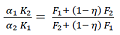
Inserting (A5) in (A7), yields
where g ≡ K1/K2 and a ≡ a1/a2. The solution of (A8) is given by
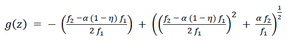 (A9)
(A9)
We thus have
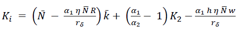
 (A10)
(A10)
Inserting (A1) in (17), we obtain
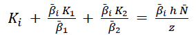
 (A11)
(A11)
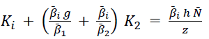
Inserting (A11) and (A10) in (18), we get
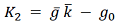 (A12)
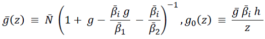
(A12)
where
From (15), we have
 (A13)
(A13)
Inserting (A1), (A4) and (10) in (A13), we obtain
 (A14)
(A14)
where
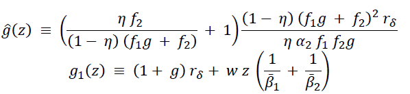
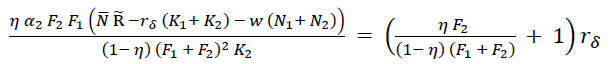
Inserting (A12) and the definition of R ̃ in (A14), we get
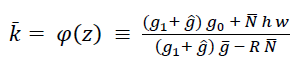 (A15)
(A15)
It is straightforward to confirm that all the variables can be expressed as functions of z by the following procedure: k ̅ by (A15) → K=k ̄N ̄ → r by (A2) → w by (A3) → K2 by (A12) → K1 by (A10) → Ki by (A11) → N1, N2 and Ni by (A1) → Fi and Fj by (A4) →R ̃ by (4) → πj by (14) → y ̂ by (4) → p by (9) → ci, cj and s by (7) → U by the definition. From this procedure and (8), we have
 (A16)
(A16)
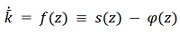
Deriving k ̅= φ(z) in time, yields
 (A17)
(A17)
 (A18)
(A18)
In summary, we have proved the lemma.
APPENDIX A-2: A computational procedure to simulate the perfectly competitive model
We still have (A1)–(A5). By (15)’ we have
 (A19)
(A19)
Inserting (A19) in (9), we get
 (A20)
(A20)
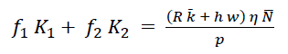
Inserting (A20) in (18), we obtain
 (A21)
(A21)
Inserting (A1) in (17), yields
 (A22)
(A22)
 (A23)
(A23)
 (A24)
(A24)
 (A25)
(A25)
From (A25), (A21), and (A20), we have
 (A26)
(A26)
Like the procedure for the lemma, we determined all the variables as functions of z by the following procedure: k ̅ by (A26) → K =k ̄N ̄ → r by (A2) → w by (A3) → p by (A24) → K1 and K2 by (A20) and (A25) → Ki by (A21) → N1, N2 and Ni by (A1) → Fi and Fj by (A4) → y ̂ by (4) → ci, cj and s by (7) → U by the definition. Like (A16)–(A18), we thus have the equation that determines the movement of z.