Sparse Subspace Clustering for Hyperspectral Images using Incomplete Pixels
Agrupación de subespacios escasos en imágenes hiperespectrales usando pixeles incompletos
Received: February 15, 2019
Accepted: May 21, 2019
Abstract
Spectral image clustering is an unsupervised method that identifies distributions of pixels using spectral information without requiring a previous training stage. Sparse subspace clustering methods assume that hyperspectral images lie in the union of multiple low-dimensional subspaces. Therefore, sparse subspace clustering assigns spectral signatures to different subspaces, expressing each spectral signature as a sparse linear combination of all the pixels, ensuring that the non-zero elements belong to the same class. Although such methods have achieved good accuracy for unsupervised classification of hyperspectral images, their computational complexity becomes intractable as the number of pixels increases, i.e., when the spatial dimensions of the image become larger. For that reason, this paper proposes to reduce the number of pixels to be classified in the hyperspectral image; subsequently, the clustering results of the missing pixels are obtained by exploiting spatial information. Specifically, this work proposes two methodologies to remove pixels: the first one is based on spatial blue noise distribution, which reduces the probability of removing neighboring pixels, and the second one is a sub-sampling procedure that eliminates every two contiguous pixels, preserving the spatial structure of the scene. The performance of the proposed spectral image clustering framework is evaluated using three datasets, which shows that a similar accuracy is achieved when up to 50% of the pixels are removed. In addition, said framework is up to 7.9 times faster than the classification of the complete data sets.
Keywords: Spectral images, Spectral clustering, Sparse subspace clustering, Sub-sampling, Image classification
Resumen
El agrupamiento de imágenes espectrales es un método no supervisado que identifica las distribuciones de píxeles utilizando información espectral, sin necesidad de una etapa previa de entrenamiento. Los métodos basados en agrupación de subespacio escasos suponen que las imágenes hiperespectrales viven en la unión de múltiples subespacios de baja dimensión. Basado en esto, la agrupación de subespacio escasos asigna firmas espectrales a diferentes subespacios, expresando cada firma espectral como una combinación lineal escasa de todos los píxeles, garantizando que los elementos que no son cero pertenecen a la misma clase. Aunque estos métodos han demostrado una buena precisión para la clasificación no supervisada de imágenes hiperespectrales, a medida que aumenta el número de píxeles, es decir, la dimensión de la imagen es grande, la complejidad computacional se vuelve intratable. Por este motivo, este documento propone reducir el número de píxeles a clasificar en la imagen hiperespectral y, posteriormente, los resultados del agrupamiento para los píxeles faltantes se obtienen explotando la información espacial. Específicamente, este trabajo propone dos metodologías para remover los píxeles: la primera se basa en una distribución espacial de ruido azul que reduce la probabilidad de que se eliminen píxeles vecinos; la segunda, es un procedimiento de submuestreo que elimina cada dos píxeles contiguos, preservando la estructura espacial de la escena. El rendimiento del algoritmo de agrupamiento de imágenes espectrales propuesto se evalúa en tres conjuntos de datos, mostrando que se obtiene una precisión similar cuando se elimina hasta la mitad de los pixeles, además, es hasta 7.9 veces más rápido en comparación con la clasificación de los conjuntos de datos completos.
Palabras clave: Imágenes hiperespectrales, agrupación espectral, agrupación de subespacios escasos, submuestreo, clasificación de imágenes
1. INTRODUCTION
Hyperspectral images (HSIs) have become a valuable tool for monitoring the Earth surface since they provide a wealth of spectral information compared to traditional RGB images [1,2]. HSIs are commonly represented as a 3D data cube, where two dimensions `(x,y)` correspond to the spatial information and the third one, to the spectral domain (`λ`). In the 3D cube, each spatial position is represented as a vector, known as a spectral signature, whose values correspond to its intensity in each spectral band. Since the amount of radiation that each material reflects, absorbs, or emits varies according to the wavelength, the spectral signature of each pixel is used as a descriptor in a wide range of applications, such as classification [
The classification of hyperspectral images can be defined as the process of assigning each pixel to one class. This task is mainly carried out under supervised methods that know some spectral pixel labels which are used in the training stage [
However, in some applications, the labeled samples are unavailable or difficult to acquire [
To date, some clustering algorithms have been used for HSIs. Specifically, they can be divided into four groups: (a) centroid-based clustering methods [13-15], (b) density-based methods [
Assuming that spectral signatures, which correspond to a land cover class, lie in the same low-dimensional subspace, a known spectral-based method called sparse subspace clustering (SSC) builds the adjacency matrix by expressing each spectral pixel as a linear combination of all spectral signatures of the scene. In addition, such solution is restricted to be sparse, which guarantees that the spectral signatures that correspond to those sparse coefficients belong to the same subspace [
For that reason, this work proposes to remove some spectral pixels from the image in order to reduce the number of points to classify. Consequently, the computational time of the clustering task is reduced. Afterward, the clustering results of the incomplete pixels are assigned using a kind of filter that selects the predominant label in a given neighborhood. Specifically, this work proposes two schemes to remove some spectral pixels. The first one is based on spatial blue noise coding [
2. SPARSE SUBSPACE CLUSTERING FOR HYPERSPECTRAL IMAGES
Let `F∈R^(L×MN)` be a hyperspectral image reorganized as `F=[f_((1) ),…,f_((MN) ) ]`, where M and N represent the spatial dimensions, `L` stands for the number of spectral bands, and `f_((k) )∈R^L` denotes the spectral signature of the `k` `-th` pixel. The SSC method assumes that the HSIs lie in the union of n low-dimensional subspaces `⋃_(i=1)^n S_i` such that each subspace corresponds to a certain land-cover class [
`min┬ C,Z` `||C||_0+λ/2||Z||_(F )^2 `
`s.t. F=FC+Z, "diag" (C)=0, C^T 1=1` (1)
where, `l_0`-norm is the number of nonzero elements of `C`; `Z`, the error matrix; and `λ`, a regularization parameter for the sparsity coefficient and noise level trade-off. The constraint "diag" `(C)=0` is used to eliminate the trivial ambiguity where a point is represented by itself, and the constraint `C^T` 1=1 ensures that it can work even in case of affine subspaces [
`min┬C,Z ||C||_1+(λ)/2||Z||_(F )^2 `
`s.t. F=FC+Z, "diag" (C)=0, `C^T` 1=1` (2)
where, the `l_1`-norm promotes sparsity, i.e., each spectral signature is represented by few pixels [
`W=|C|+|C|^T` (2)
where, `W_(i,j)` represents the similarity between the `i-th` and `j-th` pixels. Finally, to obtain the segmentation of the data into different subspaces, a weighted graph `G=(ν,ε,W)` is built, where ν denotes the set of `NM` nodes of the graph that correspond to `NM` pixels of the image; `ε⊆ν×ν`, the set of edges between the node; and `W∈R^(MN×MN)`, the weights of the edges. Then, the data is clustered by applying spectral clustering methods [8,28] over the graph G which, naively implemented, has a computational complexity `O((MN)^3 )` [
3. SPARSE SUBSPACE CLUSTERING FOR HYPERSPECTRAL IMAGES WITH INCOMPLETE PIXELS
Note that this sparse representation builds the `C` matrix using only spectral information, i.e., the sparse representation of the `k`-`t``h` pixel is the same regardless of its spatial position. Therefore, considering that land-cover materials are distributed homogeneously (i.e., contiguous pixels in a spectral image generally belong to the same material), different constraints have been applied to `C` in order to incorporate the spatial information of the scene [
For that reason, we propose to remove certain pixels from the image before solving step (2) and the spectral clustering method in order to reduce the computational time of those steps. Mathematically, the incomplete image can be represented as (4):
`F` ` ̃ ` ` = FH,` (4)
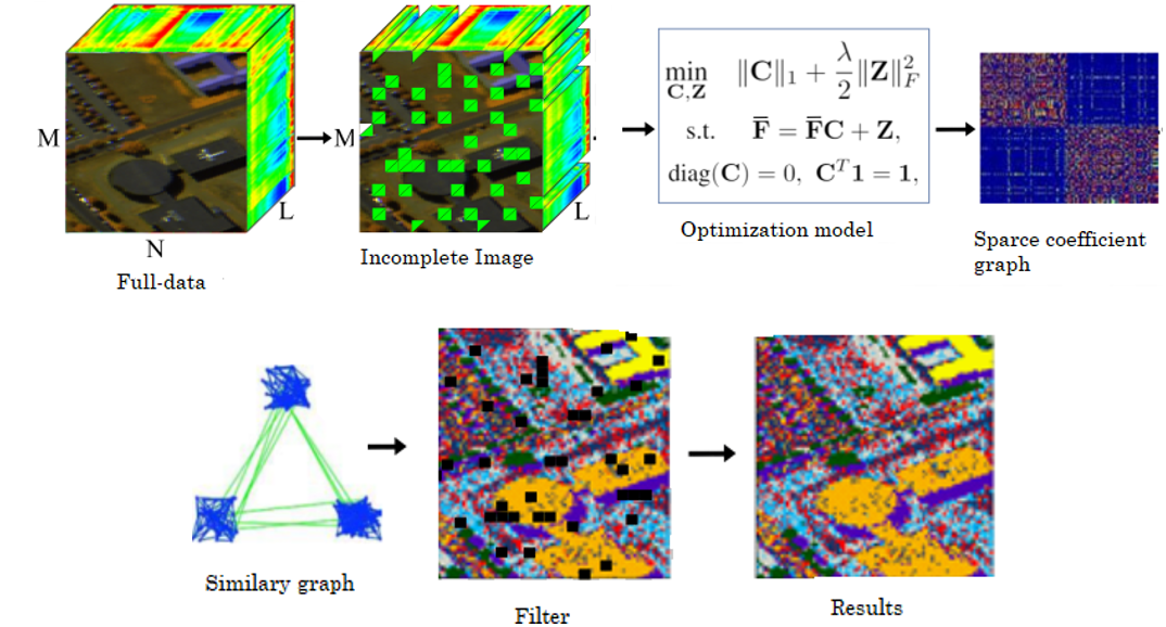
where, `F` ` ̃ ` is the incomplete image, and `H∈{0,1}^(MN×P)` is the selecting matrix that has only one non-zero value per row, with `P` as the number of preserved pixels. Therefore, the SSC model is applied to obtain the clustering results for those pixels. This segmentation can be represented in `s∈R^P`, which is a vector with the labels of the preserved pixels. In order to obtain the incomplete labels, let `s ̂ = Hs` be a vector where the missing positions are present. Then, this vector is reorganized in a matrix `S∈R^(M×N)` (see Fig. 1), where the incomplete labels are obtained applying a kind of filter that selects the predominant label in a given window; in this case, of a 3 ×3 size. Specifically, when `χ={1,...,ı}` denotes the set of ı class labels, those missing values are given by (5):
`S_(x,y)=argmax┬(χ={1,...,ı},)∑_(i=x-⌊w/2⌋)^(x+⌊w/2⌋) ∑_(j = y-⌊w/2⌋)^⌊w/2⌋ δ(S_(x,y),χ),` (5)
where `w=3` is the size of the window; ⌊.⌋, the floor function; and `δ`, the Kronecker delta function, which is 1 if the arguments are equal and 0 otherwise.
Fig. 1 represents the step-by-step of the proposed method and Algorithm 1 summarizes the computations described above. Note that the quality of the proposed methodology mainly depends on the structure of matrix `H`. For that reason, the two following sub-sections propose different strategies to design selecting matrix `H` in an efficient way.
Algorithm 1: Spectral Subspace Clustering for incomplete hyperspectral image
Input: `F, n, λ, H, p`
1. Design matrix `H`, holding `p` pixel positions
2. Extract the selected pixels as `F` `̃ ` `=HF`.
3. Solve the sparse optimization problem in (2) with the incomplete image `F` `̃ `.
4. Normalize the columns of `C` as `c_j=c_j \/\|\|c_j \|\|_∞`
5. Construct the similarity graph representing the data point `W=|C|+|C|^T.`
6. Apply spectral clustering as in [
7. Complete the non-labeled pixels using a 3 ×3 filter for the segmentation in step 6
Output: Segmentation of the data S
3.1 Design of the Selecting Matrix Based on Spatial Blue Noise Coding
An important design parameter of the selection matrix is the number of pixels that will be removed. Therefore, let `ζ_r` be the preservation ratio defined as (6):
`ζ_r=1/MN ∑_(i=1)^M ∑_(j=1)^N (H)_(i,j) =p/MN.` (6)
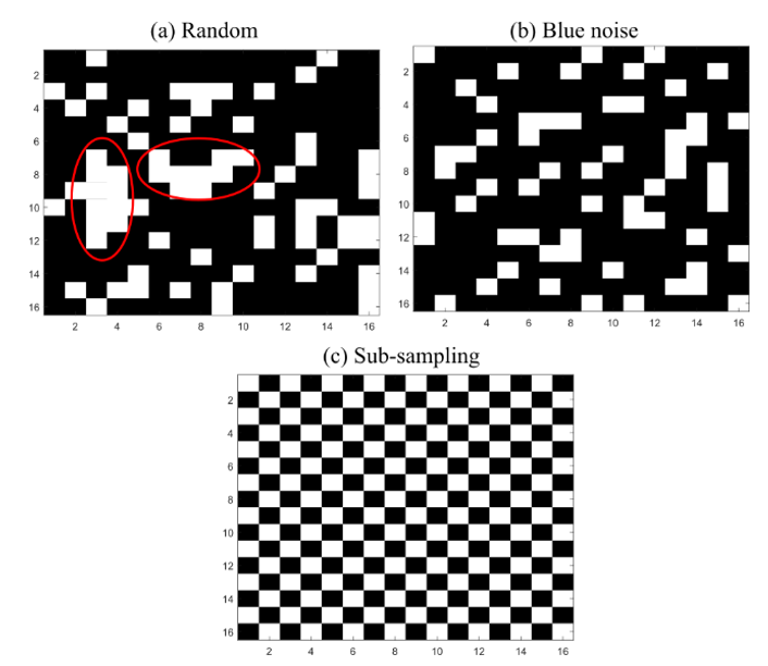
For instance, `ζ_r` = 0.2 means that 20% of the pixels would be preserved and 80% of the pixels would be removed after applying (4). A conventional selection matrix uses random entries; however, random binary codes tend to form clusters. Figure 2 (a) shows an example of a random matrix with `ζ_r` = 0.75, where matrix `H` is represented as an `M × N` matrix where white spaces mark the pixels to remove, and black represents the pixels to keep. Note that the random matrix tends to form clusters, which leads to a negative impact when the non-labeled pixels in the incomplete image are assigned using the strategy presented in Section 3. For that reason, a blue noise pixel distribution is used in order to reduce clusters and achieve uniform selected pixels, as shown in Fig. 2. (b) [
3.2 Design of the Selecting Matrix-Based Sub-sampling
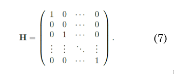
The random and spatial blue noise criteria to remove pixels do not preserve the spatial distribution of the scene after the reorganization in (4) because more rows than columns, or vice versa, can be eliminated. Therefore, SSC-based methods that incorporate the spatial information cannot be directly applied to `F` `̃ `. For that reason, a sub-sampling scheme that eliminates every two contiguous pixels and preserved the spatial structure of the images is proposed. Specifically, matrix `H` has the structure (7).
4. SIMULATIONS AND RESULTS
In this section, the performance of the proposed hyperspectral image clustering framework is evaluated. The clustering result of applying Algorithm 1 to the incomplete image is denoted as IP. The spectral Indian Pines dataset and two regions of Pavia University data set were used for these experiments. The results presented here are the average of 10 trial runs. Overall accuracy (Acc_O), average accuracy (Acc_A), and Kappa coefficients were used as quantitative performance metrics. In the tables, the metric used for each land cover class is Accuracy. All the simulations were implemented in Matlab 2017a on an Intel Core i7 3.41-Ghz CPU with 32 GB of RAM. In all the tables, the optimal value of each row is shown in bold.
4.1 Spectral image datasets
The Indian Pines hyperspectral data set, sensed by the AVIRIS sensor, has 145 × 145 pixels and 224 spectral bands [
The second scene, of Pavia University, was acquired by the Reflective Optics System Imaging Spectrometer (ROSIS) airborne sensor over an urban area of Pavia, Northern Italy. The size of the image is 610 × 340 pixels and 103 spectral bands [
The number of classes for each data set was manually fixed as an input for Algorithm 1. Additionally, parameter λ was chosen applying the formulation in [
`λ = β/γ,where γ = min┬kmax┬(k≠j)|f_k^T f_j | ,` (8)
where, γ is a parameter that directly depends on the spectral image that is used and β is a tunable parameter that was fixed for all the experiments at β=1000.
4.2 Quality of classification results vs number of eliminated pixels
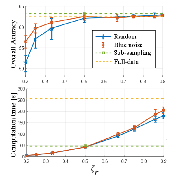
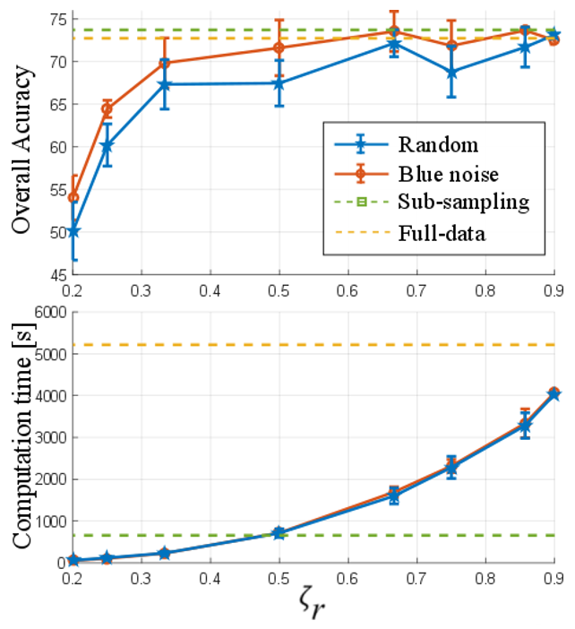
The first test was performed to show the quality of the results and the computational time using the number of eliminated pixels by means of the preservation ratio (`ζ_r`). For that purpose, the proposed methods were compared with random elimination and the complete image. The Indian Pines and Pavia University data tests were used in this test. Figure 3 and 4 show the general accuracy and the computational time obtained with the different configurations for the two data sets, respectively. Note that, in the sub-sampling method, the preservation ratio is fixed at `ζ_r= 0.5` and, with the full image, it is `ζ_r= 1`. It can be observed that, when the number of preserved pixels increases, the quality of the classification by the designed and randomized elimination schemes improves. However, the designed blue noise scheme outperforms the random selection matrix with `ζ_r≤0.5` for both data sets. In addition, the proposed methods maintain a performance comparable to the full data when more than half of the pixels are conserved. Fig. 3 and 4 also show the time spent applying different preservation ratios and a drastic increase in computational time as the number of removed pixels decreases.
4.3 Advantages of the Sub-sampling scheme
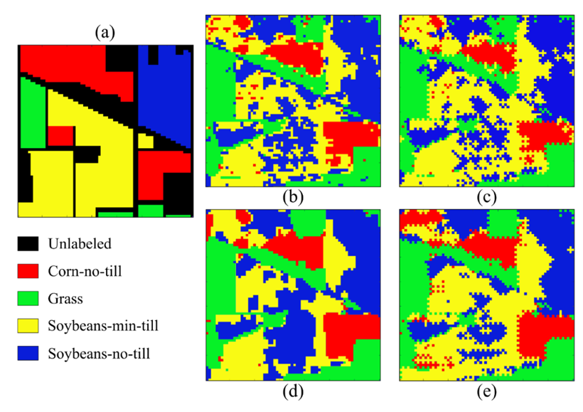
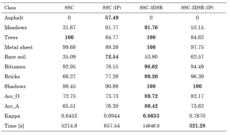
The second test shows the advantages of the sub-sampling method because SSC with spatial regularizer (SSC-SR) algorithms can be used. Therefore, the SSC with a 3D spatial regularizer (SSC-3DSR) was employed for this test [
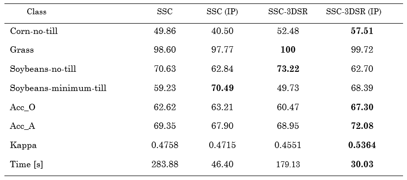
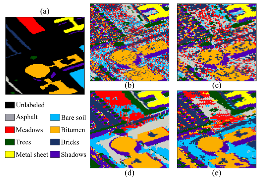
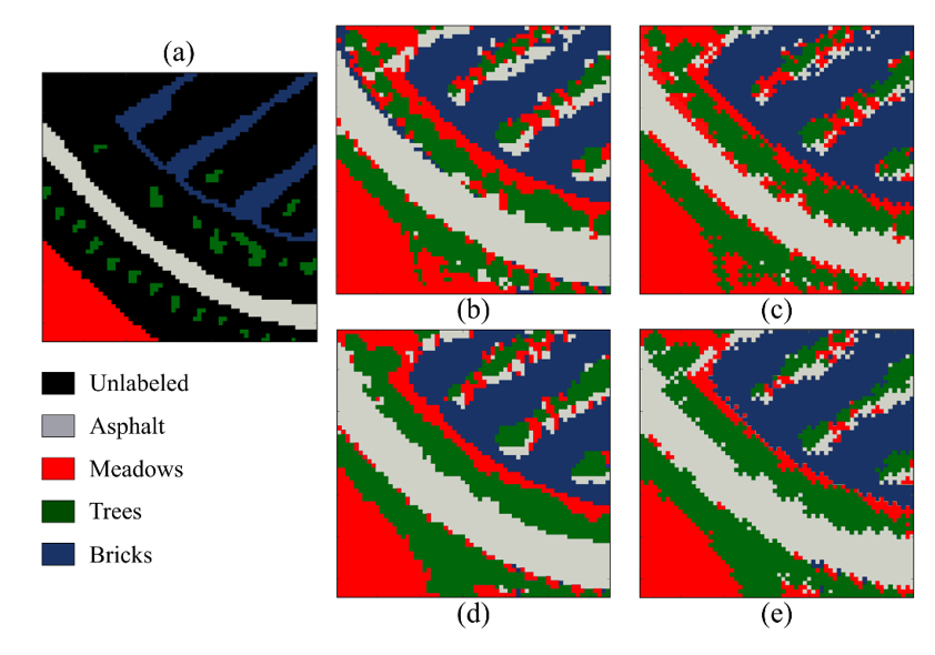
Furthermore, Figure 6 and Table 2 show the visual and numerical results of the first region of the Pavia University dataset in terms of classification accuracy. For this dataset, the best result is achieved by the SSC-3DSR without the proposed subsampling method. Moreover, the proposed scheme provides the shortest classification time, thus maintaining a good performance. Specifically, it solved the clustering problem 6.11 times faster than the other methods.
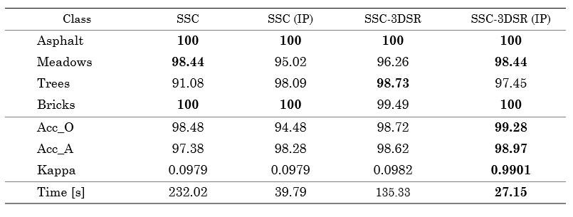
Finally, the classification performance achieved for the other region of the Pavia University dataset is shown in Fig. 7, and the quantitative results are presented in Table 3. Note that the quality is preserved, but our method is 5 times faster for this subregion of Pavia University.
5. CONCLUSIONS
A method to reduce the computational time of sparse subspace clustering for hyperspectral images was proposed in this work. Such scheme is based on the fact that some spectral pixels can be omitted in the clustering steps. Therefore, the clustering of the removed pixels is completed using a special filter that selects the most frequent value in a given neighborhood. Specifically, this work proposed two schemes to remove pixels. One is based on spatial uniform blue noise coding, and the other is a sub-sampling of every two pixels that preserves the spatial structure of the scene. In general, the results for three different datasets show that the proposed clustering achieves similar accuracy, but it is up to 7.9 times faster than the other methods. However, removing some pixels can sharply reduce classification accuracy in some images, especially when there are few pixels per class. Therefore, future work includes grouping pixels according to the spatial structure of the scene instead of eliminating them.
6. REFERENCES
- arrow_upward [1] M. Fauvel, J. Chanussot, J. A. Benediktsson, and J. R. Sveinsson, "Spectral and spatial classification of hyperspectral data using SVMs and morphological profiles," in 2007 IEEE International Geoscience and Remote Sensing Symposium, Barcelona 2007, vol. 46, no. 11, pp. 4834–4837. https://doi.org/10.1109/IGARSS.2007.4423943
- arrow_upward [2] N. M. Nasrabadi, "Hyperspectral Target Detection : An Overview of Current and Future Challenges," IEEE Signal Process. Mag., vol. 31, no. 1, pp. 34–44, Jan. 2014. https://doi.org/10.1109/MSP.2013.2278992
- arrow_upward [3] J. M. Bioucas-Dias et al., "Hyperspectral Unmixing Overview: Geometrical, Statistical, and Sparse Regression-Based Approaches," IEEE J. Sel. Top. Appl. Earth Obs. Remote Sens., vol. 5, no. 2, pp. 354–379, Apr. 2012. https://doi.org/10.1109/JSTARS.2012.2194696
- arrow_upward [4] G. Martin and J. M. Bioucas-Dias, "Hyperspectral Blind Reconstruction From Random Spectral Projections," IEEE J. Sel. Top. Appl. Earth Obs. Remote Sens., vol. 9, no. 6, pp. 2390–2399, Jun. 2016. https://doi.org/10.1109/JSTARS.2016.2541541
- arrow_upward [5] A. F. H. Goetz, G. Vane, J. E. Solomon, and B. N. Rock, "Imaging Spectrometry for Earth Remote Sensing," Science, vol. 228, no. 4704, pp. 1147–1153, Jun. 1985. https://doi.org/10.1126/science.228.4704.1147
- arrow_upward [6] Y. Liu, H. Pu, and D.-W. Sun, "Hyperspectral imaging technique for evaluating food quality and safety during various processes: A review of recent applications," Trends Food Sci. Technol., vol. 69, pp. 25–35, Nov. 2017. https://doi.org/10.1016/j.tifs.2017.08.013
- arrow_upward [7] T. Adão et al., "Hyperspectral Imaging: A Review on UAV-Based Sensors, Data Processing and Applications for Agriculture and Forestry," Remote Sens., vol. 9, no. 11, p. 1110, Oct. 2017. https://doi.org/10.3390/rs9111110
- arrow_upward [8] E. Elhamifar and R. Vidal, "Sparse Subspace Clustering: Algorithm, Theory, and Applications," IEEE Trans. Pattern Anal. Mach. Intell., vol. 35, no. 11, pp. 2765–2781, Nov. 2013. https://doi.org/10.1109/TPAMI.2013.57
- arrow_upward [9] H. Zhang, H. Zhai, L. Zhang, and P. Li, "Spectral–Spatial Sparse Subspace Clustering for Hyperspectral Remote Sensing Images," IEEE Trans. Geosci. Remote Sens., vol. 54, no. 6, pp. 3672–3684, Jun. 2016. https://doi.org/10.1109/TGRS.2016.2524557
- arrow_upward [10] J. Bacca, C. V Correa, and H. Arguello, "Noniterative Hyperspectral Image Reconstruction From Compressive Fused Measurements," IEEE J. Sel. Top. Appl. Earth Obs. Remote Sens., vol. 12, no. 4, pp. 1231–1239, Apr. 2019. https://doi.org/10.1109/JSTARS.2019.2902332
- arrow_upward [11] J. Dougherty, R. Kohavi, and M. Sahami, "Supervised and Unsupervised Discretization of Continuous Features," in Machine Learning Proceedings, California.1995 . pp. 194–202. https://doi.org/10.1016/B978-1-55860-377-6.50032-3
- arrow_upward [12] Y. Liu, H. Pu, and D.-W. Sun, "Hyperspectral imaging technique for evaluating food quality and safety during various processes: A review of recent applications," Trends Food Sci. Technol., vol. 69, no. 5, pp. 25–35, Nov. 2017. https://doi.org/10.1016/j.tifs.2017.08.013
- arrow_upward [13] S. Lloyd, "Least squares quantization in PCM," IEEE Trans. Inf. theory, vol. 28, no. 2, pp. 129–137, 1982. https://sites.cs.ucsb.edu/~veronika/MAE/kmeans_LLoyd_Least_Squares_Quantization_in_PCM.pdf
- arrow_upward [14] G. H. Ball and D. J. Hall, "ISODATA, a novel method of data analysis and pattern classification," Standford Research Institute, USA, Reporte técnico, AD 699616, 1965
- arrow_upward [15] W. Pedrycz, "Fuzzy sets in pattern recognition: Methodology and methods," Pattern Recognit., vol. 23, no. 1–2, pp. 121–146, Jan. 1990. https://doi.org/10.1016/0031-3203(90)90054-O
- arrow_upward [16] A. Rodriguez and A. Laio, "Clustering by fast search and find of density peaks," Science, vol. 344, no. 6191, pp. 1492–1496, Jun. 2014. https://doi.org/10.1126/science.1242072
- arrow_upward [17] S. Vijendra, "Efficient Clustering for High Dimensional Data: Subspace Based Clustering and Density Based Clustering," Inf. Technol. J., vol. 10, no. 6, pp. 1092–1105, Jun. 2011. https://doi.org/10.3923/itj.2011.1092.1105
- arrow_upward [18] Y. Zhong, L. Zhang, and W. Gong, "Unsupervised remote sensing image classification using an artificial immune network," Int. J. Remote Sens., vol. 32, no. 19, pp. 5461–5483 ,Aug. 2011. https://doi.org/10.1080/01431161.2010.502155
- arrow_upward [19] Y. Zhong, S. Zhang, and L. Zhang, "Automatic Fuzzy Clustering Based on Adaptive Multi-Objective Differential Evolution for Remote Sensing Imagery," IEEE J. Sel. Top. Appl. Earth Obs. Remote Sens., vol. 6, no. 5, pp. 2290–2301, Oct. 2013. https://doi.org/10.1109/JSTARS.2013.2240655
- arrow_upward [20] G. Chen and G. Lerman, "Spectral Curvature Clustering (SCC)," Int. J. Comput. Vis., vol. 81, no. 3, pp. 317–330, Mar. 2009. https://doi.org/10.1007/s11263-008-0178-9
- arrow_upward [21] C. A. Hinojosa, J. Bacca, and H. Arguello, "Spectral Imaging Subspace Clustering with 3-D Spatial Regularizer," in Imaging and Applied Optics 2018 (3D, AO, AIO, COSI, DH, IS, LACSEA, LS&C, MATH, pcAOP), Orlando. 2018. https://doi.org/10.1364/3D.2018.JW5E.7
- arrow_upward [22]C. Hinojosa, J. Bacca, and H. Arguello, "Coded Aperture Design for Compressive Spectral Subspace Clustering," IEEE J. Sel. Top. Signal Process., vol. 12, no. 6, pp. 1589–1600, Dec. 2018. https://doi.org/10.1109/JSTSP.2018.2878293
- arrow_upward [23] H. Zhang, H. Zhai, W. Liao, L. Cao, L. Zhang, and A. Pizurica, "Hyperspectral image kernel sparse subspace clustering with spatial max pooling operation," 23rd Congr. Int., vol. 41, no. B3, pp. 945–948, 2016. https://pdfs.semanticscholar.org/ace6/0a31dbcd910ff7d722625aab5896b59022e0.pdf
- arrow_upward [24] E. Elhamifar and R. Vidal, "Sparse subspace clustering," in 2009 IEEE Conference on Computer Vision and Pattern Recognition, Miami. 2009, pp. 2790–2797. https://doi.org/10.1109/CVPR.2009.5206547
- arrow_upward [25] C. V Correa, H. Arguello, and G. R. Arce, "Spatiotemporal blue noise coded aperture design for multi-shot compressive spectral imaging," J. Opt. Soc. Am. A, vol. 33, no. 12, pp. 2312–2322, 2016.
https://doi.org/10.1364/JOSAA.33.002312 - arrow_upward [26] H. Zhai, H. Zhang, L. Zhang, P. Li, and A. Plaza, "A New Sparse Subspace Clustering Algorithm for Hyperspectral Remote Sensing Imagery," IEEE Geosci. Remote Sens. Lett., vol. 14, no. 1, pp. 43–47, Jan. 2017. https://doi.org/10.1109/LGRS.2016.2625200
- arrow_upward [27] S. Boyd,N. Parikh, E. Chu, B. Peleato and J. Eckstein, "Distributed Optimization and Statistical Learning via the Alternating Direction Method of Multipliers," in Now the essence Trends machine learning, pp. 1-125, 2011. https://doi.org/10.1561/2200000016
- arrow_upward [28] A. Y. Ng, M. I. Jordan, and Y. Weiss, "On spectral clustering: Analysis and an algorithm," Adv. Neural Inf. Process. Syst., pp. 849–856, 2002. http://papers.nips.cc/paper/2092-on-spectral-clustering-analysis-and-an-algorithm.pdf
- arrow_upward [29] J. Bacca, C. A. Hinojosa, and H. Arguello, "Kernel Sparse Subspace Clustering with Total Variation Denoising for Hyperspectral Remote Sensing Images," in Imaging and Applied Optics 2017 (3D, AIO, COSI, IS, MATH, pcAOP), San Francisco,. 2017. https://doi.org/10.1364/MATH.2017.MTu4C.5
- arrow_upward [30] M. Baumgardner,L.L. Biehl., and D. Landgrebe, "220 Band AVIRIS Hyperspectral Image Data Set: June 12, 1992 Indian Pine Test Site 3." Purdue University. https://doi.org/10.4231/R7RX991C