Influence of Turbulence, Density, Phase Change, and Phase Interfaces Models on the Performance of the Numerical Simulation of a Two-Phase Closed Thermosyphon
Influencia de los modelos de turbulencia, densidad, cambio de fase e interfaz en la simulación numérica de un termosifón cerrado de dos fases
Received: Noviembre 28, 2019
Accepted: Julio 06, 2020
Abstract
A heat pipe can be considered a highly effective thermal conduction device, which is especially desirable in heat transfer operations in order to ensure high energy efficiency. However, the operation of heat pipes comprises different heat and mass transfer phenomena, such phase change, heat conduction and convection, solid-liquid and vapor-liquid surface interactions, surface vaporization, and nucleate boiling. Therefore, modelling heat pipes is a highly complex task that demands detailed knowledge of the physical phenomena involved and choosing suitable theoretical models to obtain a good representation of the real nature of the heat and mass transfer processes. In this study, some models and parameters available in the commercial CFD software ANSYS Fluent for turbulence, density, phase change, and phase interfaces were examined to determine their influence on the prediction of the heat and mass transfer in a two-phased closed thermosyphon (TPCT). The numerical results show that using a turbulence viscous model is not necessary and that a variable density model improves the temperature distribution inside the TPCT. Furthermore, using high mass and energy transfer coefficients during condensation makes the vapor remain close to the saturation temperature. Finally, a sharp interphase model is strongly recommended for this type of process.
Keywords: Thermosyphon, numerical simulation, heat pipe, phase change, Computational Fluid Dynamics.
Resumen
Un tubo de calor puede ser considerado como un dispositivo con alta conductividad térmica, el cual es frecuentemente usado en procesos de transferencia de calor para garantizar una alta eficiencia energética. Además, la operación de los tubos de calor comprende diferentes fenómenos de transferencia de calor y masa, como cambio de fase, conducción y convección, interacciones sólido-líquido y vapor-líquido, evaporación y ebullición nucleada, además de otras. Por lo tanto, el modelado de los tubos de calor es un proceso de alta complejidad, el cual requiere el conocimiento del fenómeno físico allí presente para escoger los modelos teóricos adecuados, logrando así, obtener una representación aceptable de los procesos de transferencia de masa y energía que naturalmente se presentan. En este trabajo, algunos modelos y parámetros disponibles en el software ANSYS Fluent como el modelo de viscosidad, densidad, cambio de fase e interfaz entre fases fueron analizados para determinar su influencia sobre la predicción de la transferencia de masa y energía en un termosifón cerrado de dos fases. Los resultados numéricos mostraron que, usar un modelo de viscosidad turbulenta no es necesario, un modelo de densidad variable mejora la distribución de la temperatura y que un modelo de interfaz Sharp es altamente recomendado en estos procesos.
Palabras clave: termosifón, simulation numérica, tubo de calor, cambio de fase, Dinámica de Fluidos Computacional.
1. INTRODUCTION
Heat pipes have remarkable heat transfer capacity, high thermal conductivity, and are easy to maintain.
These devices can extract heat and transport it to a condensation zone by changing the fluid phase. They are also highly efficient and their design is simple [
Such pipes have a wick through which a working fluid flows due to capillary pressure. A wickless heat pipe is called a thermosyphon, in which the working fluid flows due to gravity. Therefore, thermosyphons must operate vertically or at low inclinations.
Heat transfer in a thermosyphon is caused by the evaporation-condensation of the working fluid. The device has liquid in the evaporation zone; the heat input in this zone evaporates the liquid, and the steam goes up to the condensation zone through the adiabatic section. In the condenser, heat is deflected to the condensation fluid that remains at low temperatures. Then, the liquid film from the condensation returns to the evaporator through the pipe walls due to gravity[
Due to their high efficiency and simple operation, heat pipes are used in many engineering applications [
Therefore, it is essential to analyze the behavior of thermosyphons and their efficiency under different operating conditions.
It is difficult to experimentally describe the changing phase in a thermosyphon. For that reason, it is recommendable to study the behavior of thermosyphons using computational fluid dynamics (CFD) software. Numerical simulations achieve a huge accuracy and can reduce the time and cost of a study [
Some researchers have studied the effect of heat input, fill ratio, inclination angle, working fluid, and how these parameters affect the performance of two phase closed thermosyphons (TPCTs).
Regarding the fill ratio, Alizadehdakhel et al. [
Pulsed heat input has been studied by Kafeel et al. [
Fadhl et al. analyzed the temperature distribution in a TPCT [
Another important phenomenon in TPCTs is the geyser effect, which occurs when the liquid fill ratio is high and the heat input is low. Jouhara et al. [
Regarding the working fluid, other authors have analyzed distilled or deionized water, nanofluids, and refrigerants. Fadhl et al. [
They found that these fluids present the same behavior in a CFD simulation, and the vapor bubbles are smaller than those formed with distilled water as working fluid. Therefore, the thermal resistance of the device decreases. Ong et al. [
The effects of inclination and the fill ratio were considerable at heat inputs greater than 60 W. The highest heat transfer coefficient in condensation zone was 1200 W/m2K with a fill ratio and heat input of 0.75 and 100 W, respectively. The lowest thermal resistance was 0.17 K/W, produced with a heat input of 100 W and a fill ratio of 1.
TPCTs can operate with low angle inclinations. Zhanget et al. [
Additionally, some geometric configurations of TPCTs can be studied using CFD simulations. Fertahi et al. [
Wang et al. used CFD simulations to analyze the effects of the volumetric flow rate of the condensate fluid and the heat input on a radial wickless heat pipe [
Through CFD simulations by Wang et al. [
The effect of the condensing fluid on the temperature is significant at volumetric flow rates up to 100 ml/min.
Controllable loop heat pipes (CLHPs) are thermosyphons with control valves in the vapor and liquid lines. These devices are used in refrigerators to extract heat from their compartments. The effect of non- condensable gases on CLHPs has been studied by Cao et al. [
Azzolin et al. analyzed a TCTP with integrated water storage through numerical simulations [
Zhang et al. studied an air conditioning system for data centers using simulations [
Wang et al. implemented the Lee model to simulate heat and mass transfer in CFD software [
The implementation of the UDF in the model aimed to properly simulate the nucleation phenomenon according to the overheating temperatures with the modification of the relaxation factor in the equations. In the numerical simulation with the original Lee model, the liquid pool temperature in the evaporation zone remained close to the saturation temperature, while in the numerical simulation with the modified model the liquid pool and the steam bubbles presented overheating temperatures. The simulation with the modified model represented more accurately the bubble formation observed experimentally.
Despite the number of numerical simulations performed to represent the operation of a TPCT, the literature lacks studies about the most suitable models and parameters to reproduce the different heat and mass transfers occurring in this type of devices because these phenomena are hard to observe experimentally. Therefore, this study aims to deepen our understanding of some models available in a commercial CFD code (ANSYS Fluent), which could be applied to the numerical simulation of a TPCT in order to obtain an accurate representation of the physical phenomena governing the operation of such device.
Particularly, the models and parameters of turbulence, density, phase change, and phase interfaces were modified and the results were analyzed to determine the feasibility of the application of those models and parameters to the simulation of a TPCT.
2. METHODOLOGY
2.1 Theoretical model
ANSYS Fluent software was used for the numerical simulation of a TPCT. The Volume of Fluid (VOF) model was used to simulate the multi-phase flow. All the phases present in the simulation were considered immiscible [
∝l+∝v= 1 (1)
Where ∝𝑙 and ∝𝑣 are the liquid fraction and vapor volume, respectively. If the cell is full of liquid, then ∝𝑙= 1; but, if it’s full of steam, ∝𝑣= 1.
The density in a computational cell is defined as (2):
𝜌 =∝𝑣 𝜌𝑣 +∝𝑙 𝜌𝑙 (2)
Where 𝜌𝑣 and 𝜌𝑙 correspond to the vapor and liquid density, respectively. The continuity equation for VOF model is (3), (4):
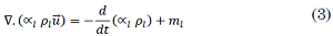
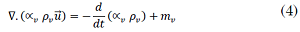
Where 𝑢⃗ represents the average velocity, and 𝑚𝑣 and 𝑚𝑙 are the mas flows due to evaporation-condensation respectively. The momentum equation including the volume fraction terms is set as (5):
Where I represent the unit tensor, 𝑝 denotes the pressure and 𝑔 the gravity 𝜇 denotes the viscosity, this value is in function of volume fraction in a computational cell as (6):
μ= ∝v μv+∝l μl (6)
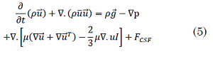
FCSF determine the volumetric surface tension This term was proposed by Brackbill [
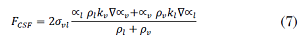
Where 𝜎𝑣𝑙 is the surface tension coefficient (8).
The energy equation is:
Where 𝑇 is the mixture temperature. The thermal conductivity in each cell is calculated through the volume fraction (9):
k=∝l kl+∝v kv (9)
Where 𝑘𝑙 and 𝑘𝑣 are the energy transfer rates of liquid and steam, respectively. The specific energy of the system is (10):
The terms 𝑒𝑙 and 𝑒𝑣 are calculated in function of the specific heat (11) and (12):
el=cp,l (T-Tsat) (11)
ev=cp,v (T-Tsat) (12)
Where 𝑐𝑝,𝑙 and 𝑐𝑝,𝑣 are the specific heats for liquid and vapor, respectively.
Fluent´s mass and energy transfer model is the Lee model [
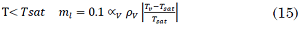
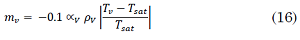
The energy transfer between phases is (17) and (18):
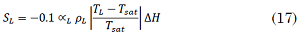
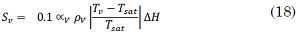
Where ∆𝐻 is the vaporization enthalpy.
2.2 Development of the simulation
The geometry of the TPCT, the mesh and the simulation was performed in ANSYS 18.1. The model geometry was drawn in DesingModeler. A 2D model was proposed and the specifications are shown in Table1.
| Variable | Value |
| Material | Copper |
| Total length | 440 mm |
| Evaporator length | 250 mm |
| Condensation zone length | 190 mm |
| Outer diameter | 12.78 mm |
| Inner diameter | 10.32 mm |
| Wall thickness | 1.23 mm |
| Working fluid | Deionized water |
| Condensate fluid | Water |
The mesh was designed with Meshing in ANSYS Workbench. A cut cell method was used to structure the mesh. The cells have an initial spacing of 0.1 mm and a growth factor of 1.2 near the inner wall to simulate the condensate bubbles.
The resultant mesh is shown in Fig. 1.
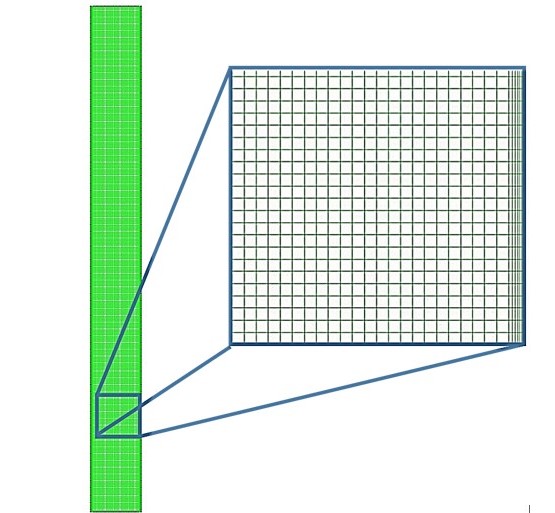
A total of 58,800 grids were used for the computational calculation. The wall thickness was created as a boundary condition in ANSYS Fluent, as shown in Fig. 1.
In Fluent, a transient solution scheme was selected to simulate the operation of the TPCT. The pressure-based solver was selected for this simulation. The VOF model was chosen for the numerical simulation with two Eulerian phases.
A temperature-dependent density correlation was proposed according to data in liquid and steam tables based on values obtained from [
ρl = -0.0038T 2 + 2.2623T + 655.27 (19)
The vapor density was calculated using the ideal gas law. The surface tension coefficient was defined through (20) based on data obtained from [
σlv = -3x10⁻⁷T 2 - 0.0001T + 0.0756 (20)
2.2.1 Boundary conditions
A constant heat flux of 6973.925 W/m2 was imposed in the evaporation zone. In the top and the bottom caps, the imposed heat flux was 0, i.e., they were considered adiabatic surfaces. The condenser zone wall The condenser zone wall had a constant output heat flux of 9176.22 W/m2.
A non-slip boundary was defined on the inner wall of all the zones in the TPCT.
2.2.2. Solution methods
The SIMPLE algorithm was chosen for the Pressure-Velocity coupling, and the schemes for the discretization were first-order upwind for momentum and energy equations, Geo- Reconstruct for volume of fraction equation, and PRESTO for pressure. The time step size was 5x10⁻⁴ s, and the convergence criteria was based on residuals around 10-6 or lower for energy and 10-3 or lower for the other equations.
2.2.3 Initial parameters
Some initial parameters and models were ideal gas density, a laminar viscosity model, a mass and energy transfer coefficient of 0.1, and sharp interface modelling. However, changes were made to these parameters and models during the simulation to achieve convergence and fitting of the experimental data.
For example, viscosity was shifted to a urbulent k-Ω model, sharp interface modelling was shifted to disperse interface, and the mass and energy transfer coefficient was varied between 0.1 and 100. Other parameters and models remained unchanged.
2.3 Experimental procedure
To validate the CFD simulation, an experimental evaluation was conducted.
The experimental set up is shown in Fig. 2. type J. Five thermocouples were located in the evaporation zone, three thermocouples in the condensation zone, and two thermocouples in the inlet and outlet of the condensate fluid.
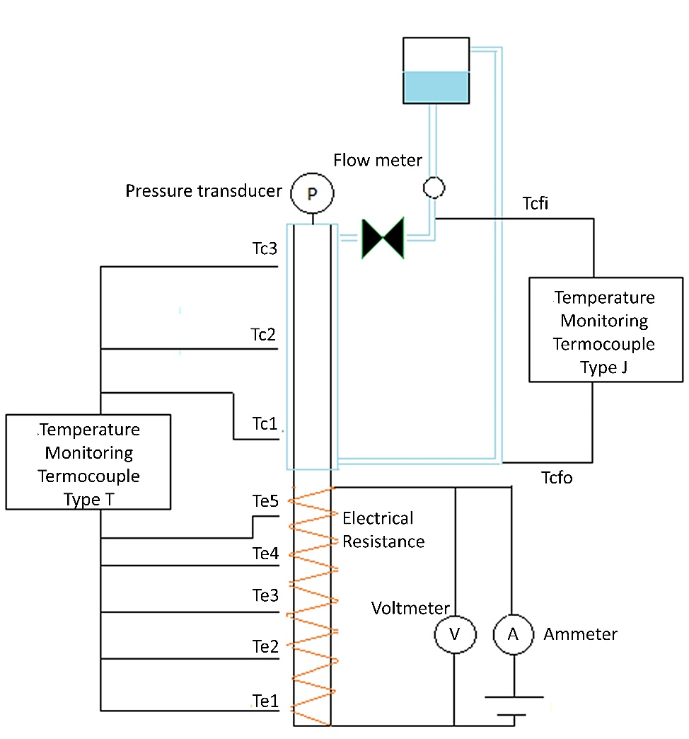
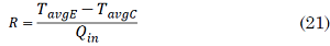
A pressure transducer was used in the device to monitor the pressure, and a submersible pump condenser increased, too. The effect of this difference on the thermal performance of the TPCP was considered using the thermal resistance, which was calculated employing the average temperatures in the device’s zone at each supplied power through (21):
Was used to ensure a constant volumetric flow rate of cooling fluid in the condensation zone. Also, thermostatic bath was used to ensure a constant temperature of 25 °C for the cooling fluid.
The power input in the evaporator was simulated through a direct current power supply and an electrical resistance.
The power input was calculated using Watt’s law, the power input was calculated using Watt’s law and the measurements of current and voltage.
The output power in the condensation zone was calculated using Newton’s heat transfer law.
3. RESULTS
3.1 Experimental evaluation
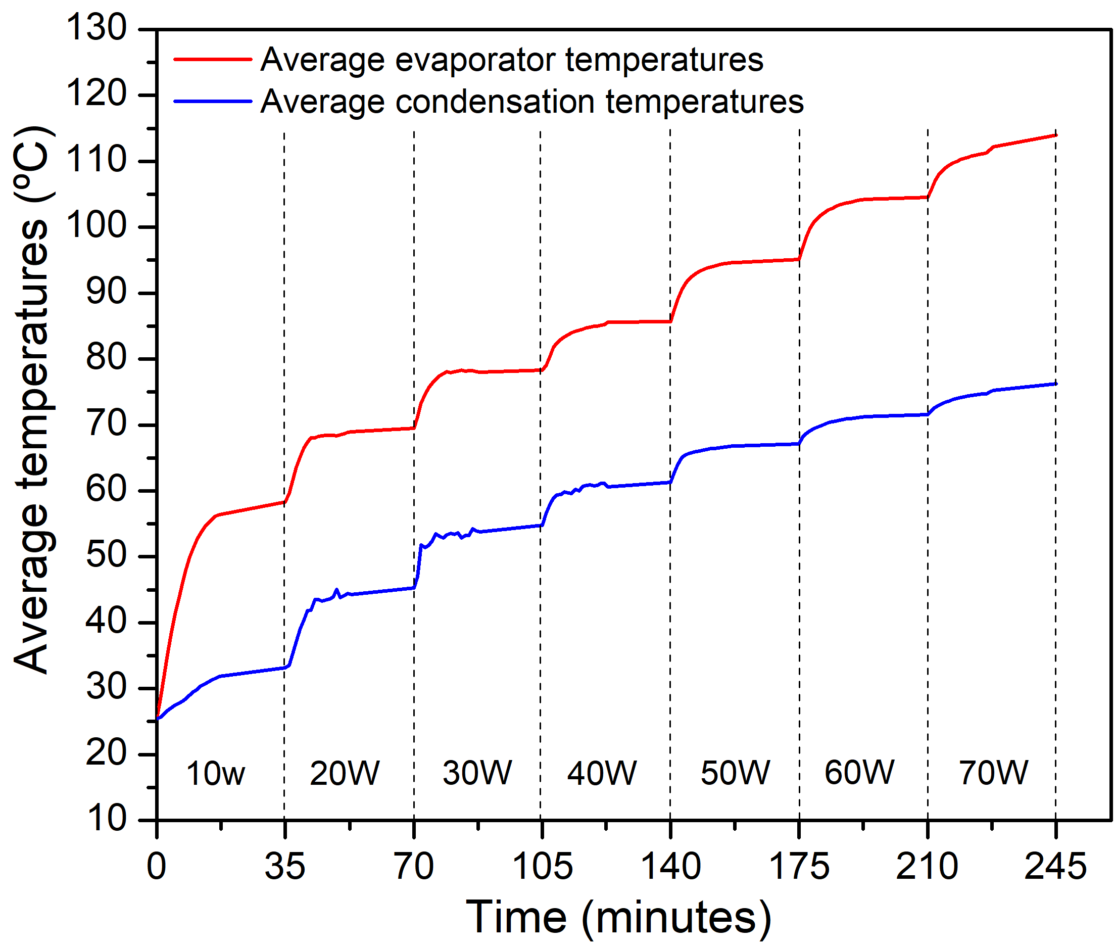
Four tests were conducted with the same conditions: an initial vacuum pressure of 71.11 kPa, an input power of 10W initially, and a 10 W increase every 35 minutes up to 70 W.
The results in Fig. 3 show that the temperature rises as the input power increases. After each power increase, the temperature rose up to a steady state after 19 minutes. Between 19 and 35 minutes, the changes in average temperature in the device’s zones were not significant, between 19 and 35 minutes, the changes in average temperature in the device’s zones were not significant, and it is considered the saturation temperature because an increase in the pressure inside the device due to evaporation caused an increase in the saturation temperature. In Fig. 3, the temperature curve on the bottom shows the average temperatures in the condensation zone, while the upper curve represents the average temperatures in the evaporation zone.
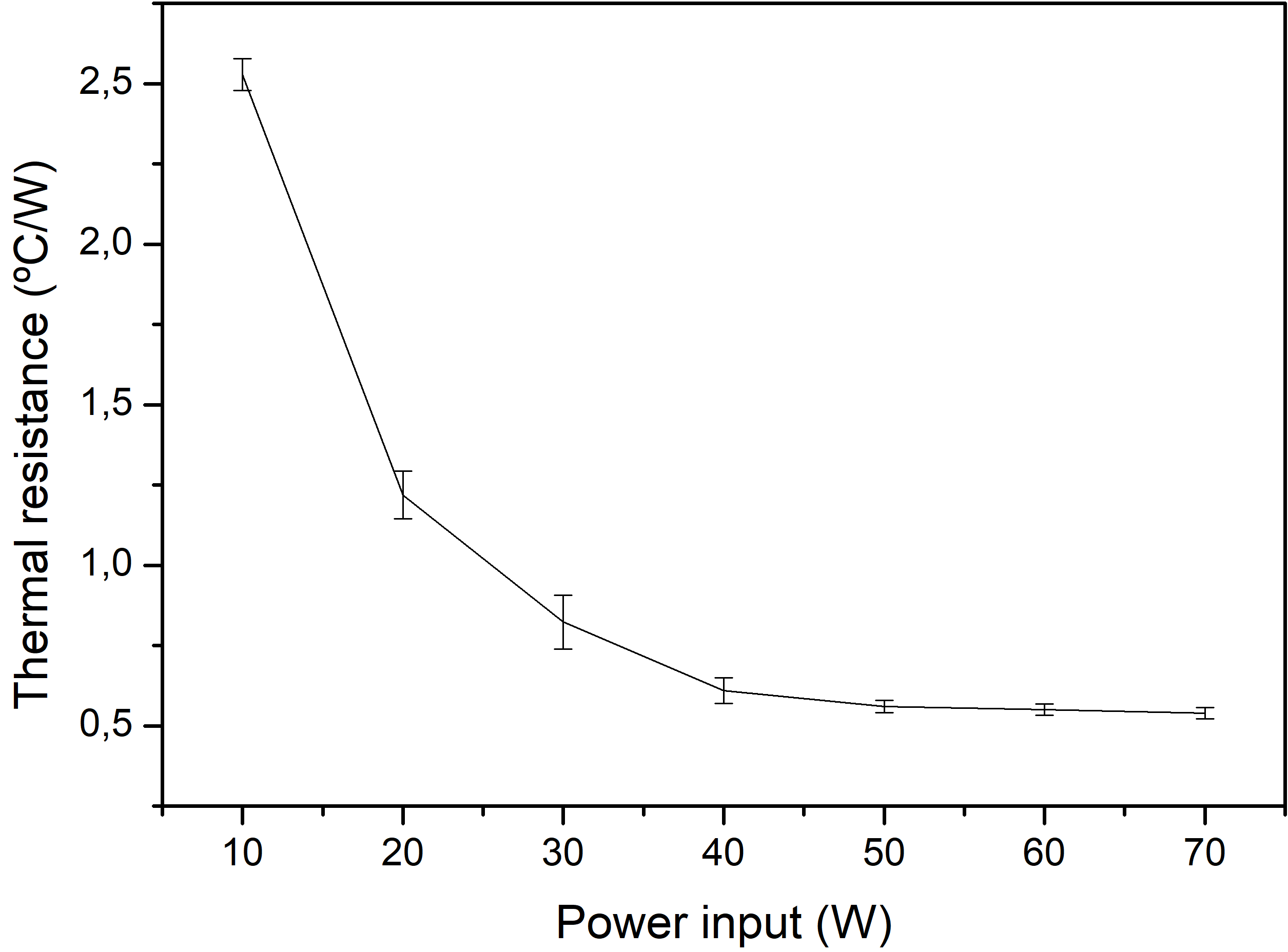
The experimental results in Fig. 4 show that the thermal resistance of the TPCT decreased as the power input increased. Furthermore, the thermal resistance shows an asymptotic behavior close to 0.5 (°C/W). In Fig. 3, the temperature difference between the evaporation and condensation zones is greater at high input powers. Equation (19) shows a proportionality with such difference, while input power is inversely proportional to thermal resistance. Then, as can be seen in Fig. 4, the higher input power was the most influential factor in the increase in temperature differences in the device.
3.2 CFD model validation
For the validation, the thermosyphon in the CFD simulation had the geometry shown in Table 1. 50 W were imposed as the boundary condition in the evaporation and condensation zones. The time step was 5x10⁻⁴ s.
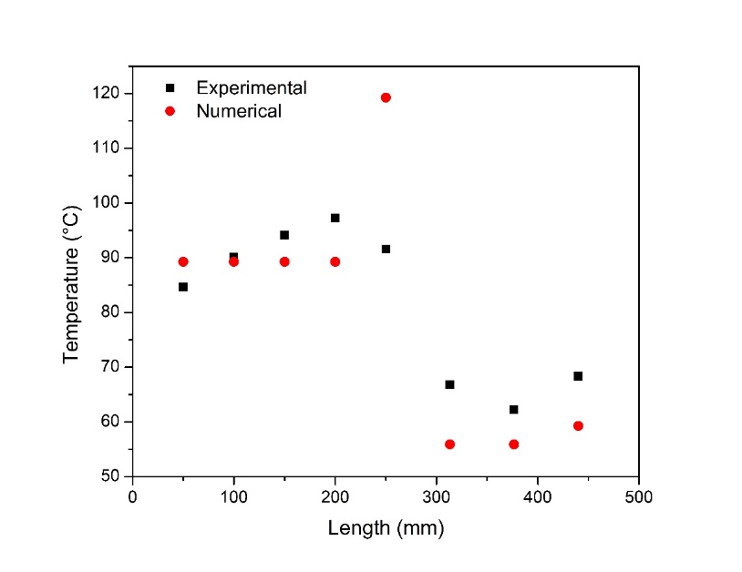
Along the length of the thermosyphon, there was a good agreement in temperature values between the experiments and the CFD simulations.
The results are shown in Fig. 5. The deviation of 25 °C in the central zone is believed to be due to the fact that the numerical model is not able to predict the geyser phenomenon that occurs in the real thermosyphon, which helps to stabilize the wall temperature. Therefore, future work should aim to overcome this limitation of numerical simulations.
3.3 Numerical Simulation
A numerical simulation with phase change is a fluid flow problem of special attention since when the immiscible phases are dependent each other, it is easy to obtain divergence. That is why it is necessary to properly define the physical phenomenon there. A series of numerical simulations were performed to determine the behavior of the fluid flow, the average temperatures and the heat transfer in the device. The process consisted in the variation of some parameters mentioned below, while the other parameters remained constant. The parameter varied where:
3.3.1 Turbulence model
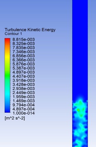
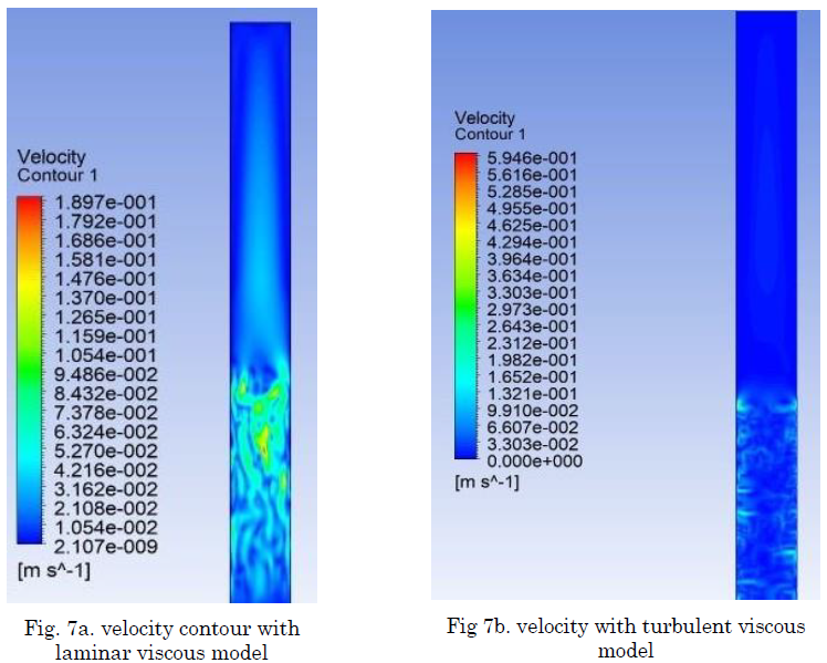
ANSYS Fluent has different models such as k-Ɛ model and k-ɷ model for simulation of turbulence. Two regimes were analyzed through the laminar and kɷ models, for laminar and turbulent regime, respectively. The results obtained for both models were the similar. Besides, Fluent allows to observe the kinetic energy dissipation. For the turbulent model implemented, the kinetic energy dissipation has a low value as can be seen in the contour in the evaporation zone in Fig. 6. The highest value 8.82x10⁻³ m. /s. was obtained in the liquid pool, while, in other zones in the device, the turbulent kinetic energy is negligible. In Fig. 7, it can be seen the velocity contours for the laminar and turbulence viscous model, where it is possible to observe that the velocity profile with turbulence viscous model corresponds to low velocities between 0 and 10-1 meters per second, which confirms the velocity scale of the laminar viscosity model.
3.3.2 Density model
Density plays an important role when the buoyancy is present inside the physic phenomenon. In a TPCT, the saturated vapor goes up in the center of the pipe while the liquid from condensation returns to the bottom of the device on the tube walls. Due to high temperatures, it is possible that the vapor reaches high velocities, causing an increase of Courant´s number. This number is the ratio between the computational cell length and the flow velocity. When this number is greater than 0.25, the simulation diverges. By the other hand, high speeds produce, in the same way, high pressures, causing divergence in equations or poor convergence.
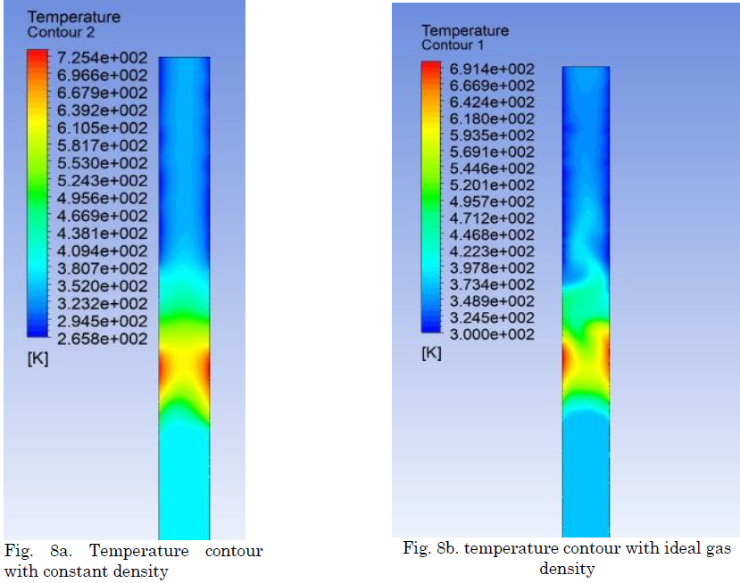
In the present study, two simulations were performed with two density models for vapor: constant density and ideal gas law density. With constant density, the vapor velocity rising is low, but the high temperatures predominate in evaporation section where there is no liquid. Also, with constant density model for vapor, a maximum speed of 0.7 meters per second is observed in the evaporation zone, while, in the condensation zone, the vapor reaches low speeds, which prevents the temperature homogenization in the condensation zone and increases the temperature differences between the device´s zones, which increases the thermal resistance.
Using the ideal gas law for the gas phase, the temperature is evenly distributed along the pipe, and the velocity of vapor is higher than with constant steam density. Fig. 8a and Fig. 8b, shows the temperature contours for both cases.
3.3.3 Energy and mass transfer coefficient calculated using the phase change
The 0.1 energy and mass transfer coefficient used in the Lee model [
Imposing a constant temperature as boundary condition in condensation zone, it is possible to obtain a constant output heat rate, and the cool temperature remains constant only in the cell near the wall pipe.
With coefficients between 0.1 and 1, the simulation remains in a steady state, but it is not possible to see a condensate film.
Around the first seconds, the output heat rate is high due to temperature differences.
Then, the vapor reaches thermal equilibrium with the wall, causing a low output heat rate. Therefore, the coefficient of mass flow and energy sources for evaporation must always be low because, otherwise, it causes divergence.
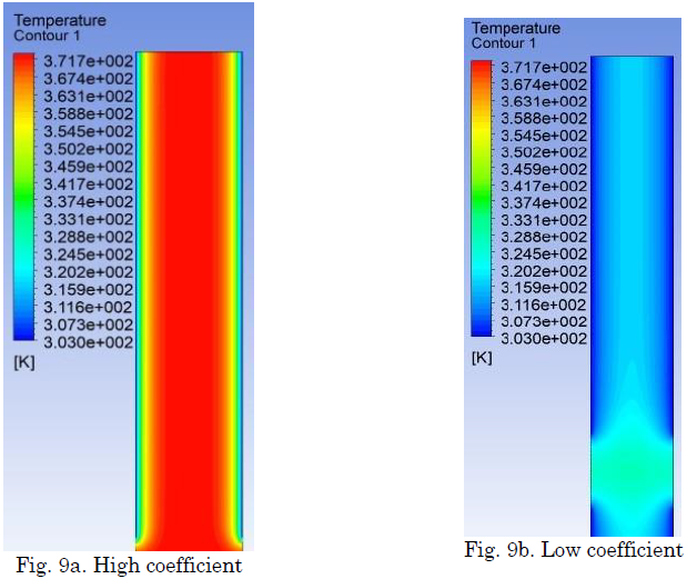
Fig. 9 shows the temperature profile produced with different mass and energy transfer coefficients in phase change.
3.3.4 Interface Modelling
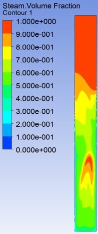
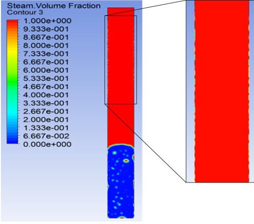
Two options for interface modelling were evaluated: sharp and disperse interface. Choosing the right type of interface is important because this parameter controls the mixing of phases and the movement of each phase relative to the other. In a disperse interface, two or more phases are interpenetrating, while the sharp interface is appropriate when a distinct interface is present between the phases. Fig. 10 and Fig. 11 were obtained using the disperse and sharp interfaces, respectively. In the case of the disperse interface, vapor was mixed with the liquid phase in all the zones of the device when the phase change occurred, while the sharp interface restricted the condensing fluid to the walls of the device. Therefore, in order to reproduce the phase change phenomenon in a TPCT, a sharp interface is highly recommended.
4. CONCLUSIONS
A numerical simulation of the operation of a TPCP was performed to visualize the effect of choosing some parameters offered in ANSYS Fluent.
According to the results, using a turbulence viscous model is not necessary because the velocity profiles were the same with laminar and turbulent models.
Additionally, using a turbulence model requires a lot of computation time.
Therefore, the physical phenomenon inside the TPCT can be better represented with a laminar viscous model. In terms of the density model, a variable density model improved the temperature distribution inside the device because it allowed for vapor buoyancy.
The phase change during condensation should be an isothermal process for vapor that remains at the center of the pipe.
With high mass and energy transfer coefficients during condensation, the vapor remains close the saturation temperature. Finally, the disperse interphase model did not show good results because the phases were mixed when the phase changed, while the sharp interphase model allowed the phases to be immiscible with a different interface between both phases, which is closer to the physical phenomenon that takes place inside TPCTs.
5. ACKNOWLEDGMENTS
The authors would like to acknowledge to Instituto Tecnológico Metropolitano for financial support to the Researchers and Innovators Youngs program (Resolution No. 000277 of 04 MAR 2019). Research Group of Advanced Materials and Energy - MATyER is also acknowledged.
CONFLICTS OF INTEREST
None declared.
6. REFERENCES
- arrow_upward [1] A. Alizadehdakhel ; M. Rahimi; A. Abdulaziz Alsairafi, “CFD modeling of flow and heat transfer in a thermosyphon,” Int.Commun. Heat Mass Transf., vol. 37, no. 3, pp. 312–318, Mar. 2010. https://doi.org/10.1016/j.icheatmasstransfer.2009.09.002
- arrow_upward [2] B. Fadhl; L. C. Wrobel; H. Jouhara, “Numerical modelling of the temperature distribution in a two-phase closed thermosyphon,” Appl. Therm. Eng., vol. 60, no. 1–2, pp. 122–131, Oct. 2013. https://doi.org/10.1016/j.applthermaleng.2013.06.044
- arrow_upward [3] K. Kerrigan; H. Jouhara; G. E. O’Donnell; A. J. Robinson, “Heat pipe-based radiator for low grade geothermal energy conversion in domestic space heating,” Simul. Model. Pract. Theory, vol. 19, no. 4, pp. 1154–1163, Apr. 2011. https://doi.org/10.1016/j.simpat.2010.05.020
- arrow_upward [4] Y.-C. Weng; H.-P. Cho; C. C. Chang; S. L. Chen, “Heat pipe with PCM for electronic cooling,” Appl. Energy, vol. 88, no. 5, pp. 1825–1833, May 2011. https://doi.org/10.1016/j.apenergy.2010.12.004
- arrow_upward [5] X. Ping Wu; P. Johnson; A. Akbarzadeh, “Application of heat pipe heat exchangers to humidity control in air-conditioning systems,” Appl. Therm. Eng., vol. 17, no. 6, pp. 561–568, Jun. 1997. https://doi.org/10.1016/S1359-4311(96)00058-0
- arrow_upward [6] Z. Xu; Y. Zhang; B. Li; C. C. Wang; Y. Li, “The influences of the inclination angle and evaporator wettability on the heat performance of a thermosyphon by simulation and experiment,” Int. J. Heat Mass Transf., vol. 116, pp. 675–684, Jan. 2018. https://doi.org/10.1016/j.ijheatmasstransfer.2017.09.028
- arrow_upward [7] K. Kafeel; A. Turan, “Simulation of the response of a thermosyphon under pulsed heat input conditions,” Int. J. Therm. Sci., vol. 80, pp. 33–40, Jun. 2014. https://doi.org/10.1016/j.ijthermalsci.2014.01.020
- arrow_upward [8] H. Jouhara; B. Fadhl; L. C. Wrobel, “Three-dimensional CFD simulation of geyser boiling in a two- phase closed thermosyphon,” Int. J. Hydrogen Energy, vol. 41, no. 37, pp. 16463–16476, Oct. 2016. https://doi.org/10.1016/j.ijhydene.2016.02.038
- arrow_upward [9] B. Fadhl; L. C. Wrobel; H. Jouhara, “CFD modelling of a two- phase closed thermosyphon charged with R134a and R404a,” Appl. Therm. Eng., vol. 78, pp. 482–490, Mar. 2015. https://doi.org/10.1016/j.applthermaleng.2014.12.062
- arrow_upward [10] K. S. Ong; G. Goh; K. H. Tshai; W. M. Chin, “Thermal resistance of a thermosyphon filled with R410A operating at low evaporator temperature,” Appl. Therm. Eng., vol. 106, no. 5, pp. 1345–1351, Aug. 2016. https://doi.org/10.1016/j.applthermaleng.2016.06.080
- arrow_upward [11] S. ed-D. Fertahi; T. Bouhal; Y. Agrouaz; T. Kousksou; T. El Rhafiki; Y. Zeraouli, “Performance optimization of a two-phase closed thermosyphon through CFD numerical simulations,” Appl. Therm. Eng., vol. 128, pp. 551–563, Jan. 2018. https://doi.org/10.1016/j.applthermaleng.2017.09.049
- arrow_upward [12] W.-W. Wang; Y. Cai; R.-Z. Liu; F.-Y. Zhao; D. Liu, “Experimental and numerical investigations of a radial heat pipe for waste heat recovery,” Appl. Therm. Eng., vol. 154, pp. 602– 613, May 2019. https://doi.org/10.1016/j.applthermaleng.2019.03.06
- arrow_upward [13] X. Wang; H. Yao; J. Li; Y. Wang; Y. Zhu, “Experimental and numerical investigation on heat transfer characteristics of ammonia thermosyhpons at shallow geothermal temperature,” Int. J. Heat Mass Transf., vol. 136, pp. 1147–1159, Jun. 2019. https://doi.org/10.1016/j.ijheatmasstransfer.2019.03.080
- arrow_upward [14] J. Cao; G. Pei; M. Bottarelli; C. Chen; D. Jiao; J. Li, “Effect of non-condensable gas on the behaviours of a controllable loop thermosyphon under active control,” Appl. Therm. Eng., vol. 146, pp. 288– 294, Jan. 2019. https://doi.org/10.1016/j.applthermaleng.2018.09.132
- arrow_upward [15] M. Azzolin; A. Mariani; L. Moro; A. Tolotto; P. Toninelli; D. Del Col, “Mathematical model of a thermosyphon integrated storage solar collector,” Renew. Energy, vol. 128, no. Part A, pp. 400–415, Dec. 2018. https://doi.org/10.1016/j.renene.2018.05.057
- arrow_upward [16] H. Zhang; S. Shao; C. Tian, “Simulation of the Thermosyphon Free Cooling Mode in an Integrated System of Mechanical Refrigeration and Thermosyphon for Data Centers,” Energy Procedia, vol. 75, pp. 1458–1463, Aug. 2015. https://doi.org/10.1016/j.egypro.2015.07.260
- arrow_upward [17] X. Wang; Y. Wang; H. Chen; Y. Zhu, “A combined CFD/visualization investigation of heat transfer behaviors during geyser boiling in two-phase closed thermosyphon,” Int. J. Heat Mass Transf., vol. 121, pp. 703–714, Jun. 2018. https://doi.org/10.1016/j.ijheatmasstransfer.2018.01.005
- arrow_upward [18] C. W. Hirt; B. D. Nichols, “Volume of Fluid (VOF) Method for the Dynamics of Free Boundaries,” J. Comput. Phys., vol. 39, no. 1, pp. 201–225, Jan. 1981. https://doi.org/10.1016/0021-9991(81)90145-5
- arrow_upward [19] J. U.Brackbill; D. B. Kothe; C. Zemach, “A Continuum Method for Modeling Surface Tension,” J. Comput. Phys., pp. 335–354, Vol. 100, no. 2 Jun. 1992. https://doi.org/10.1016/0021-9991(92)90240-Y
- arrow_upward [20] Y. A. Cengel; M. A. Boles, “A Pressure Iteration Scheme for Two-Phase Flow Modeling,” in Computational Methods for Two-Phase Flow and Particle Transport, McGrawHill, 1980. https://doi.org/10.1142/9789814460286_0004
- arrow_upward [21] Y. A. M. a. B. Çengel, Termodinámica, 7th ed. México, 2009
- arrow_upward [22] R. Mott, Mecánica de fluídos. Pearson: México, 2006
7. CONTRIBUTIONS
1 Review of the state of art, meshing and executions of numerical simulations, results analysis and article writing.
2 Content review and English writing. Simulations planning and results analysis.