Modeling Cutting Forces in High-Speed Turning using Artificial Neural Networks
Modelado de las fuerzas de corte en el torneado de alta velocidad utilizando redes neuronales artificiales
Received: August 24, 2020
Accepted: December 18, 2020
Available: April 22, 2021
L. W. Hernández-González; D. A. Curra-Sosa; R. Pérez-Rodríguez; P. D. C. Zambrano-Robledo, “Modeling Cutting Forces in High-Speed Turning using Artificial Neural Networks”, TecnoLógicas, vol. 24, nro. 51, e1671, 2021. https://doi.org/10.22430/22565337.1671
Highlights
Abstract
Cutting forces are very important variables in machining performance because they affect surface roughness, cutting tool life, and energy consumption. Reducing electrical energy consumption in manufacturing processes not only provides economic benefits to manufacturers but also improves their environmental performance. Many factors, such as cutting tool material, cutting speed, and machining time, have an impact on cutting forces and energy consumption. Recently, many studies have investigated the energy consumption of machine tools; however, only a few have examined high-speed turning of plain carbon steel. This paper seeks to analyze the effects of cutting tool materials and cutting speed on cutting forces and Specific Energy Consumption (SEC) during dry high-speed turning of AISI 1045 steel. For this purpose, cutting forces were experimentally measured and compared with estimates of predictive models developed using polynomial regression and artificial neural networks. The resulting models were evaluated based on two performance metrics: coefficient of determination and root mean square error. According to the results, the polynomial models did not reach 70% in the representation of the variability of the data. The cutting speed and machining time associated with the highest and lowest SEC of CT5015-P10 and GC4225-P25 inserts were calculated. The lowest SEC values of these cutting tools were obtained at a medium cutting speed. Also, the SEC of the GC4225 insert was found to be higher than that of the CT5015 tool.
Keywords: Cutting forces, Specific energy consumption, High-speed turning, Artificial neural networks.
Resumen
Las fuerzas de corte son variables muy importantes para el rendimiento del mecanizado, ya que afectan la rugosidad de la superficie, la vida útil de la herramienta de corte y el consumo de energía. La reducción del consumo de energía eléctrica de los procesos de fabricación no solo beneficia económicamente a los fabricantes, sino que también mejora su comportamiento medioambiental. Muchos factores, como el material de la herramienta de corte, la velocidad de corte y el tiempo de mecanizado, afectan la fuerza de corte y el consumo de energía de la máquina. En la actualidad, muchas investigaciones se han realizado sobre el consumo energético de las máquinas herramienta. Sin embargo, la investigación sobre torneado de acero al carbono a alta velocidad es escasa. En este trabajo se estudiaron los efectos de los materiales de las herramientas de corte y su velocidad sobre las fuerzas de corte y el consumo específico de energía en el torneado en seco de alta velocidad de acero AISI 1045. Las fuerzas de corte se determinaron experimentalmente y se compararon con las estimaciones de los modelos predictivos desarrollados mediante regresión polinomial y redes neuronales artificiales. Los modelos obtenidos fueron evaluados según métricas de desempeño como el coeficiente de determinación y la raíz del error cuadrático medio, donde los modelos polinomiales no superaron el 70% en la representación de la variabilidad de los datos. Se determinó la velocidad de corte y el tiempo de mecanizado relacionados con el mayor y menor consumo de energía de las plaquitas CT5015-P10 y GC4225-P25. Los valores más bajos de consumo de energía de estas herramientas se alcanzaron para la velocidad de corte intermedia. Además, la plaquita GC4225 presentó un mayor consumo que la herramienta CT5015.
Palabras clave: Fuerzas de corte, Consumo específico de energía, Torneado de alta velocidad, Redes Neuronales Artificiales.
1. INTRODUCTION
Turning is one of the most common and useful machining operations performed in factories. Several studies have been developed to improve the machinability of materials and estimate the various cutting parameters using different modeling and optimization techniques to obtain the best machining characteristics (e.g., surface roughness, tool wear, and cutting forces).
Cutting forces are an important variable in machining, as they could indicate excessive wear of the cutting tool. This, in turn, negatively influences the surface roughness of the machined workpiece, its productivity and energy consumption, and the costs associated with the process. In addition, cutting forces are usually employed to calculate the energy consumed during the cutting process, an aspect of great relevance today. However, little research has been conducted to optimize the specific energy consumption in the high-speed turning of medium carbon steel.
In [
Likewise, the cutting forces, operation stability, cutting power, and energy consumption in the machining process could also increase.
In recent years, many renowned universities, companies, and international organizations have conducted extensive research on the energy consumption of machine tools [
In [
Nonetheless, these authors did not consider the optimization of cutting parameters in their study. Lin [
Davies et al. [
Moreover, Quan et al. [
Ozlu et al. [
Özel et al. [
Furthermore, Stachurski et al. [
Qasim et al. [
Rahim et al. [
For their part, Xie et al. [
Paul et al. [
Makhfi et al. [
Karabulut [
Dahbi et al. [
Hanief et al. [
In addition, these authors demonstrated that the ANN model was able to predict the cutting forces more accurately than the regression one and that cutting force was largely influenced by feed rate.
Arnold et al. [
Peng et al. [
Curra et al. [
According to this literature review, there are few studies into the turning of carbon steel dealing with the optimal selection of cutting parameters based on cutting forces and energy consumption.
Thus, the purpose of this study is to investigate the effects of cutting tool materials and cutting speed on cutting forces and Specific Energy Consumption (SEC) during the dry high-speed turning of AISI 1045 steel. The cutting forces are experimentally measured and compared with the results of a supervised learning algorithm. The effectiveness of the proposed model is validated based on the accuracy in terms of functional fitting using two performance metrics (mean squared error and the coefficient of determination). The model selected for each insert allowed us to obtain the values of the SEC in each of the established cutting regimes.
2. MATERIALS AND METHODS
2.1 Workpiece material
In this study, AISI-SAE 1045 steel was selected as the workpiece material. Its characteristics are presented in [
2.2 Characteristics of inserts
Coated carbide GC4225-P25 and uncoated cermet CT5015-P10 inserts were used during the experiment to calculate cutting forces. Cutting tools were manufactured by Sandvik and their characteristics are specified in [
2.3 Machine tool
The workpieces were machined on a MILLTRONICS CNC lathe machine with a maximum spindle speed of 3000 r/min and a spindle power of 9/7.5 kW. The samples had a diameter of 80 mm and a length of 300 mm. The length/diameter ratio was kept lesser than 10 to avoid chatter during machining. The workpieces were mounted between the chuck and the tailstock.
2.4 Formulation
In this study, the dependence between cutting forces and cutting parameters is determined by means of a neural network that represents the functional relationship between them. The following relationships are used to calculate the rotational speed (1) and the test duration (2):
 (1)
(1)
where
n: rotational speed (r/min);
vc: cutting speed (m/min);
D: workpiece diameter (mm).
 (2)
(2)
where
T: test duration (min);
L: workpiece machining length (mm);
f: feed (mm/r).
Since the power consumption of machine tools is dominated by the power consumption of the spindle system, this article will focus on the latter [
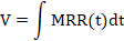
SEC is the energy consumed by the spindle system when machining 1 cm3 of material. As a result, the model can be expressed as (3) [
 (3)
(3)
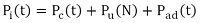
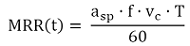
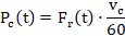
Here, Ec represents the energy consumption of the spindle system during the machining process (4); V, the volume of material removal (5); Pi(t), the input power of the spindle system at t (6); MRR(t), the material removal rate at t (7); Pc(t), the cutting power of the machining operation (8); Pu(N), the idle power (9); Pad(t), the additional load loss of the spindle system (10); asp, the depth of cut; and T, the test duration. Functions Pc(t), Pu(N), and Pad(t) are, respectively, given by [
 (4)
(4)
 (5)
(5)
 (6)
(6)
 (7)
(7)
 (8)
(8)
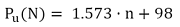 (9)
(9)
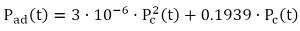 (10)
(10)
Finally, Fr(t) is the resultant cutting force (11); and Fx(t), Fy(t), and Fz(t), the components of the cutting force over time, which will be predicted by the designed model using a supervised learning algorithm.
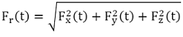 (11)
(11)
3. EXPERIMENTAL DESIGN AND SETUP
3.1 Experimental data and software
This study measures the cutting forces of the coated carbide GC4225-P25 and uncoated cermet CT5015-P10 inserts during the dry high-speed turning of AISI 1045 steel at different cutting speeds and machining times.
The cutting depth (asp = 0.5 mm) and the feed (f = 0.1 mm/r) were kept constant during all tests. The experiment was conducted using two cutting tool materials (CT5015-P10 and GC4225-P25), three cutting speeds (vc = 400 m/min, vc = 500 m/min, vc = 600 m/min), and five test durations (T1, T2, T3, T4, and T5.). A full factorial design with two replications was implemented to obtain the data [
The cutting forces were measured using a piezoelectric dynamometer (manufactured by Kistler) with a data acquisition card PC16024. National Instruments LabVIEW software was employed to analyze the data. Through an interface board, the analog signals obtained with the dynamometer were converted into digital signals.
The software used for data processing was MATLAB 2017b [
From the experimental test during the turning of AISI 1045 steel, data on cutting speed (vc), test duration (T), machining (observation) time (t), number of passes (np), and position of the cutting tool on the workpiece (pc) were recorded for each insert. These data were entered into MATLAB as vectors consisting of five independent variables (vc, T, t, np, and pc) and three dependent variables that denote the cutting forces (Fx, Fy, and Fz).
Table 1 shows the experimental design matrix used in this study and from which the cutting forces were measured.
| Insert | vc (m/min) | T (min) | Number of records |
| CT5015-P10 | 400 | 2 | 1136 |
| 4 | 2442 | ||
| 6 | 2520 | ||
| 8 | 1224 | ||
| 10 | 1234 | ||
| 500 | 1 | 727 | |
| 2 | 1265 | ||
| 3 | 1266 | ||
| 4 | 640 | ||
| 5 | 656 | ||
| 600 | 0.6 | 384 | |
| 1.2 | 737 | ||
| 2 | 812 | ||
| 3 | 648 | ||
| 4 | 666 | ||
| GC4225-P25 | 400 | 2 | 1226 |
| 4 | 2451 | ||
| 6 | 2658 | ||
| 8 | 1267 | ||
| 10 | 1249 | ||
| 500 | 1 | 644 | |
| 2 | 1249 | ||
| 3 | 1250 | ||
| 4 | 655 | ||
| 5 | 646 | ||
| 600 | 0.6 | 442 | |
| 1.2 | 772 | ||
| 2 | 765 | ||
| 3 | 633 | ||
| 4 | 512 |
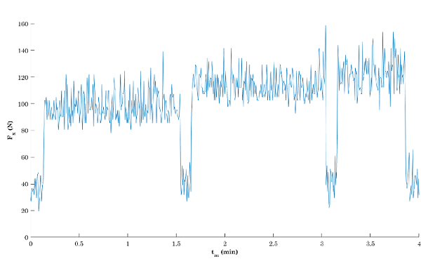
3.2 Cutting force patterns
Measuring cutting forces in machining operations makes it possible to identify behavior patterns across the different stages of the process (i.e., start, cutting, return, cutting, return, cutting, and so on) until the test duration is completed. Figure 1 shows the cutting force values per record.
Given the need to predict behavior patterns in machining operations, tools that can extract complex linear and non-linear relationships from a data set, without prior knowledge of the phenomenon being modeled, are required. In this regard, regression techniques have proven to be effective in index estimation given their potential for function fitting. In this study, multiple regression and ANN methods were used to model the relationships between cutting parameters and cutting forces.
3.3 Multiple linear regression analysis
Due to the regularities in the distribution of the shear force values, their complexity may prevent one from obtaining a predictive model through multiple regression. This is mainly due to the density of records in each cutting regime and the variability between measurements given uncontrolled process vibrations and other external effects.
However, different models were obtained considering polynomials whose degrees ranged from one to five. In all the cases, the estimation accuracy was found to be insufficient according to the standardized values in the field of study for the two performance metrics employed: coefficient of determination (R2) and Root Mean Squared Error (RMSE).
3.4 Neural network configuration
When considering several designs of Function Fitting Neural Networks (FFNN) (shown in Table 2), the best results in terms of their performance in the processing of the datasets of both inserts were obtained when similar topologies were used.
| Components | Values |
| Number of neurons in the hidden layer | 10–25 |
| Transfer functions of neurons in the hidden layer | Hyperbolic tangent sigmoid and logarithmic sigmoid |
| Transfer functions of neurons in the output layer | Poslin and purelin |
| Performance function | Mean squared error and mean absolute error |
| Distribution of the dataset for training, validation, and testing | {0.6; 0.2; 0.2}, {0.7; 0.15; 0.15}, {0.8; 0.1; 0.1} |
| Selection of records for training, selection, and testing | Random and uniform |
| Training algorithm | Levenberg–Marquardt backpropagation, scaled conjugated gradient backpropagation, and resilient backpropagation |
When designing the model, a manageable number of topologies were considered, and the rest were discarded because of poor performance. From each topology, the 10 best models obtained with the same initial conditions were identified. Finally, a FFNN topology consisting of an input layer with 5 neurons, an output layer with 3 neurons, and a hidden layer with 25 neurons (Figure 2). Here, I. (1 ≤ i ≤ 5) denotes the neurons of the input layer; Hh (1 ≤ h ≤ 25), the neurons of the hidden layer, where b. represents its bias and wih are the weights of the connections between the input and hidden layers; and O0 (1 ≤ o ≤ 3), the neurons of the output layer, where B0 represents its bias and Who are the weights of the connections between the hidden and output layers.
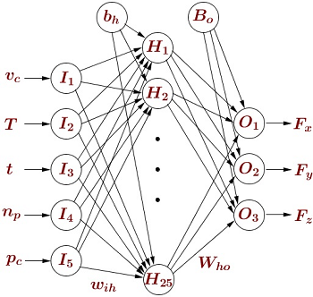
The combination of the best results considered, as activation functions, the hyperbolic tangent sigmoid and the linear in the hidden and output layers, respectively, as well as the Levenberg–Marquardt backpropagation training algorithm.
The 16 357 records for the CT5015-P10 insert were distributed as follows: 60 % for training, 20 % for validation, and 20 % for testing, as such distribution provided the least error. Similarly, records were uniformly selected: for subsets of five consecutive records, three records, one record, and one record were randomly chosen for training, validation, and testing, respectively.
In the case of the 16 419 records for the GC4225-P25 insert, the distribution that turned out to be the best was 70 %, 15 %, and 15 %. For every 20 consecutive records, 14 records, 3 records, and 3 records were randomly chosen for training, validation, and testing, respectively.
4. RESULTS AND DISCUSSION
After conducting an extensive experimentation to obtain the predictive models, which exhibited the best performances in both supervised learning approaches, the superiority of the model developed with FFNN was confirmed. The complexity present in the relationship between the analyzed variables was not even 90 % described by the polynomial regression models. According to Table 3, such models are a poor fit to the experimental data and are also characterized by high RMSE values.
| Insert | Target | Polynomial degree | R2 | RMSE (N) |
| CT5015-P10 | Fx | 1 | 0.0695 | 35.7 |
| 2 | 0.3750 | 29.3 | ||
| 3 | 0.4530 | 27.4 | ||
| 4 | 0.6110 | 23.1 | ||
| 5 | 0.6240 | 22.8 | ||
| Fy | 1 | 0.0332 | 24.3 | |
| 2 | 0.3060 | 20.6 | ||
| 3 | 0.3540 | 19.9 | ||
| 4 | 0.5110 | 17.3 | ||
| 5 | 0.5290 | 17.0 | ||
| Fz | 1 | 0.0686 | 73.2 | |
| 2 | 0.4540 | 56.1 | ||
| 3 | 0.5450 | 51.2 | ||
| 4 | 0.6850 | 42.7 | ||
| 5 | 0.6970 | 41.9 | ||
| GC4225-P25 | Fx | 1 | 0.1050 | 43.2 |
| 2 | 0.3570 | 36.7 | ||
| 3 | 0.4270 | 34.7 | ||
| 4 | 0.6350 | 27.7 | ||
| 5 | 0.6700 | 26.4 | ||
| Fy | 1 | 0.2180 | 44.8 | |
| 2 | 0.5490 | 34.0 | ||
| 3 | 0.6320 | 30.8 | ||
| 4 | 0.7560 | 25.1 | ||
| 5 | 0.7730 | 24.2 | ||
| Fz | 1 | 0.0752 | 66.5 | |
| 2 | 0.3170 | 57.2 | ||
| 3 | 0.4440 | 51.6 | ||
| 4 | 0.6730 | 39.6 | ||
| 5 | 0.6960 | 38.2 |
On the contrary, the FFNN models were found to better fit the behavior patterns of the cutting forces based on the parameters considered, since their support structure is designed to describe the complex variability in the variables under study, as is the case of this research.
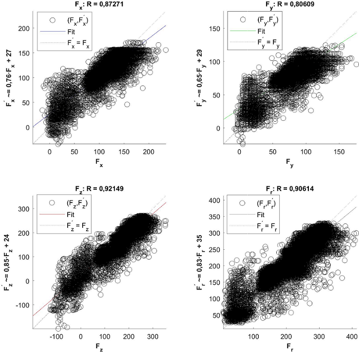
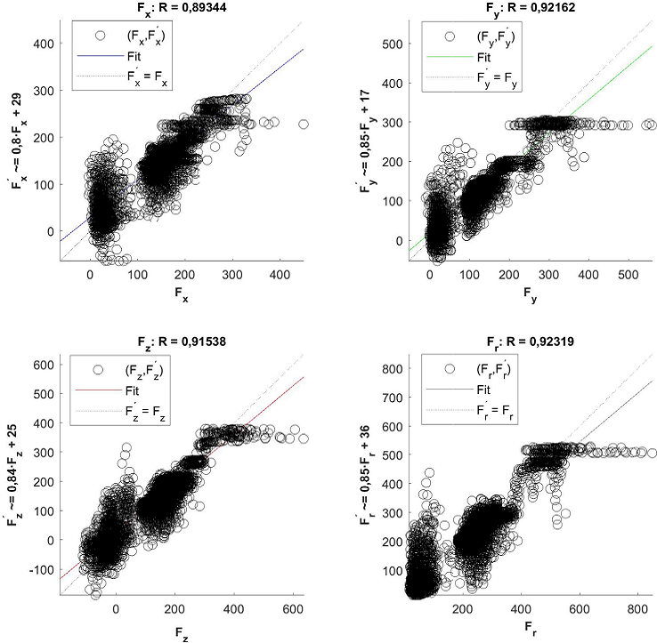
For the designed FFNN models, Figures 3 and 4 show the fitting level of the components of the estimated cutting forces (y-axis) to the components of the experimental cutting forces (x-axis). For each insert, the point cloud is over the equality line, which is confirmed by the fact that the value of the regression coefficient (R) is close to 1.
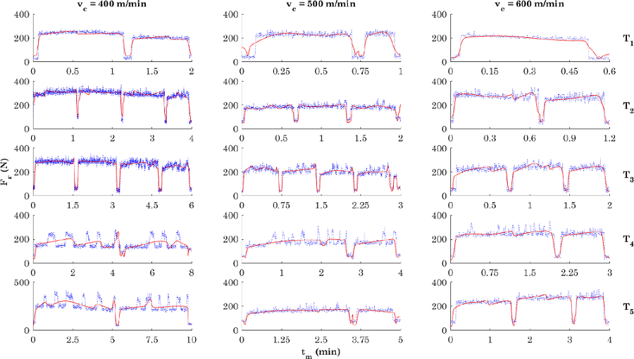
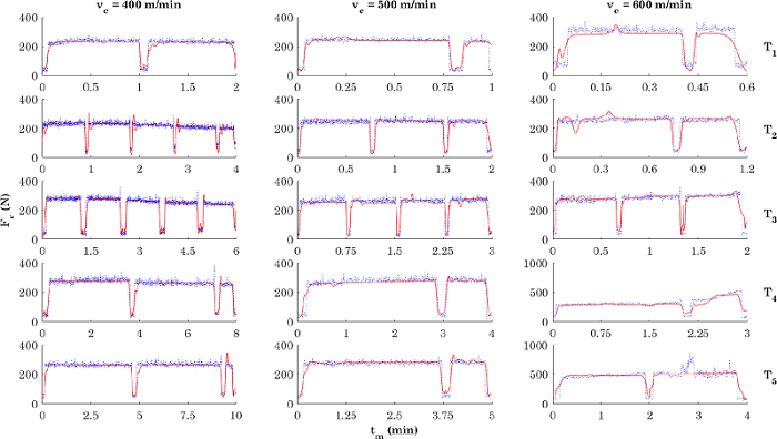
Figures 5 and 6 illustrate the accuracy of the efficiency indexes (i.e., error value or R-adjustment) based on the values of the resultant cutting force. The blue point cloud represents the experimental values; and the red line, the values estimated by the model in each cutting regime under analysis. The cutting speed levels and test duration levels are displayed in columns and rows, respectively.
The observed proximity between the resultant cutting forces led to the SEC values presented in Table 4. According to this table, there is a small difference between the mean values of the experimental and estimated SEC in all the experiment combinations. In addition, in most cases, the values of the deviations induced by the error are smaller for the estimated results. Therefore, the range of values for the estimated SEC constitutes a subset of the range of values for the experimental SEC.
| Insert | vc (m/min) | T (min) | Experimental SEC (J/cm3) | Estimated SEC (J/cm3) |
| CT5015-P10 | 400 | 2 | 12 731 ± 741 | 12 698 ± 615 |
| 4 | 14 650 ± 312 | 14 650 ± 269 | ||
| 6 | 13 878 ± 272 | 13 841 ± 244 | ||
| 8 | 11 630 ± 139 | 11 592 ± 98 | ||
| 10 | 13 675 ± 166 | 13 627 ± 119 | ||
| 500 | 1 | 12 305 ± 1 827 | 12 388 ± 1 381 | |
| 2 | 11 929 ± 408 | 11 842 ± 434 | ||
| 3 | 12 340 ± 430 | 12 275 ± 436 | ||
| 4 | 11 738 ± 286 | 11 641 ± 246 | ||
| 5 | 11 412 ± 150 | 11 318 ± 141 | ||
| 600 | 0.6 | 11 784 ± 2 796 | 11 718 ± 2 315 | |
| 1.2 | 13 695 ± 1 267 | 13 671 ± 1 152 | ||
| 2 | 12 703 ± 812 | 12 677 ± 671 | ||
| 3 | 13 124 ± 504 | 13 081 ± 473 | ||
| 4 | 13 297 ± 389 | 13 286 ± 367 | ||
| GC4225-P25 | 400 | 2 | 12 996 ± 627 | 12 916 ± 528 |
| 4 | 12 916 ± 226 | 12 864 ± 270 | ||
| 6 | 13 374 ± 309 | 13 411 ± 281 | ||
| 8 | 13 797 ± 194 | 13 783 ± 177 | ||
| 10 | 13 791 ± 132 | 13 719 ± 126 | ||
| 500 | 1 | 12 939 ± 1 574 | 13 031 ± 1 381 | |
| 2 | 13 337 ± 646 | 13 350 ± 683 | ||
| 3 | 13 631 ± 519 | 13 528 ± 460 | ||
| 4 | 13 798 ± 459 | 13 671 ± 380 | ||
| 5 | 13 860 ± 324 | 13 952 ± 294 | ||
| 600 | 0.6 | 13 988 ± 3 919 | 13 633 ± 3 111 | |
| 1.2 | 13 367 ± 1 233 | 13 466 ± 1 370 | ||
| 2 | 13 981 ± 892 | 14 161 ± 693 | ||
| 3 | 15 295 ± 736 | 14 998 ± 606 | ||
| 4 | 18 577 ± 910 | 18 653 ± 627 |
The highest SEC for the CT5015-P10 insert occurred at a cutting speed of 400 m/min with a test duration of 4 min; and for the GC4225-P25 insert, at a cutting speed of 600 m/min with a test duration of 4 min. The lowest SEC for the CT5015-P10 insert occurred at a cutting speed of 500 m/min with a test duration of 5 min; and for the GC4225-P25 insert, at a cutting % higher than that for the CT5015-P10 insert. These results show the complexity of the machining process, which depends on a considerable number of factors.
The coefficients of determination and the root mean squared error of the polynomial models did not exceed 80 % in the representation of the variability of the data. Those of the models developed with neural networks, however, exceeded 90 %, which represents an acceptable performance in the functional fitting of the shear forces. These findings reveal the good level of reliability of the FFNN models in predicting SEC under various machining conditions to further adopt the necessary energy-saving strategies.
These models could support engineers' decision-making by providing them with knowledge-based assistance. As auxiliary tools, they could be used to explore the behavior of different cutting regimes in terms of adopting resource-saving measures.
5. CONCLUSIONS
In this paper, the cutting forces, and the Specific Energy Consumption (SEC) during the dry high-speed turning of AISI 1045 steel were modeled using a function fitting neural network topology. For this purpose, we described the experiments and data sets derived from them, which formed the knowledge base learned by the model developed in MATLAB. The estimation of the SEC under the different cutting conditions proved to be highly accurate, which was corroborated by the values of the performance metrics and the graphical representations.
The cutting forces were experimentally measured and compared with the estimates of the predictive models developed using polynomial regression and artificial neural networks. The resulting models were evaluated based on two performance metrics (coefficient of determination and root mean squared error). The polynomial models were found not to exceed 80 % in the representation of the variability of the data, while the models developed with neural networks exceeded 90 %, which is an acceptable accuracy in terms of the functional fitting of the cutting forces. These results are consistent with those reported in [
These findings show the good level of reliability of the FFNN models in predicting SEC under various machining conditions to further adopt the necessary energy-saving strategies.
The highest SEC for the CT5015-P10 insert occurred at a cutting speed of 400 m/min with a test duration of 4 min; and for the GC4225-P25 insert, at a cutting speed of 600 m/min with a test duration of 4 min. The lowest SEC for the CT5015 insert occurred at a cutting speed of 500 m/min with a test duration of 5 min; for the GC4225 insert, at a cutting speed of 400 m/min with a test duration of 4 min. Likewise, the intermediate cutting speed (vc = 500 m/min) produced the lowest SEC values for both inserts. Moreover, the SEC for the GC4225 insert was 8.943 % higher than that for the CT5015 insert.
These results confirm the complexity of the machining process, which depends on a considerable number of factors. Therefore, further work needs to be done with a higher number of replicates and a greater range of cutting speeds, as well as with other cutting tool materials.
6. ACKNOWLEDGMENTS
The authors would like to thank PRONABES for providing a postgraduate research scholarship at the Universidad Autónoma de Nuevo León (UANL) in México. We are also grateful for the financial support from the Centro de Desarrollo, Investigación e Innovación Tecnológica (UANL) in Monterrey and the Instituto Tecnológico y de Estudios Superiores de Monterrey (México, Campus of Monterrey), for all the facilities to develop this research. We also want to thank the Department of Mechanical Engineering of the University of Holguín, for the offered support.
CONFLICTS OF INTEREST
The authors declare that there is no conflict of interest.
7. REFERENCES
- arrow_upward [1] H. Schulz; T. Moriwaki, “High-Speed Machining,” CIRP Annals, vol. 41, no. 2, pp. 637-643, 1992. https://doi.org/10.1016/S0007-8506(07)63250-8
- arrow_upward [2] J. Xie; F. Liu; H. Qiu, “An integrated model for predicting the specific energy consumption of manufacturing processes,” Int. J. Adv. Manuf. Technol., vol. 85, pp. 1339–1346, Nov. 2015. https://doi.org/10.1007/s00170-015-8033-y
- arrow_upward [3] R. Tanaka; Y. Yamane; K. Sekiya; N. Narutaki; T. Shiraga, “Machinability of BN free-machining steel in turning,” Int. J. Mach. Tools Manuf., vol. 47, no. 12-13, pp. 1971–1977, Oct. 2007. https://doi.org/10.1016/j.ijmachtools.2007.02.003
- arrow_upward [4] B. Denkena; R. Ben-Amor; L. De-Leon-García; J. Dege, “Material specific definition of the high speed cutting range,” Int. J. Mach. Mach. Mater., vol. 2, no. 2, pp. 176-185, May. 2007. https://doi.org/10.1504/IJMMM.2007.013781
- arrow_upward [5] W. S. Lin, “The reliability analysis of cutting tools in the HSM processes,” Archives of Materials Science and Engineering, vol. 30, no. 2, pp. 97-100, Apr. 2008. http://www.amse.acmsse.h2.pl/vol30_2/3028.pdf
- arrow_upward [6] M. Davies; A. L. Cooke; E. R. Larsen, “High bandwidth thermal microscopy of machining AISI 1045 steel,” CIRP Ann., vol. 54, no. 1, pp. 63-66, Jun. 2005. https://doi.org/10.1016/S0007-8506(07)60050-X
- arrow_upward [7] S. A. Iqbal; P. T. Mativenga; M. A. Sheikh, “Characterization of machining of AISI 1045 steel over a wide range of cutting speeds. Part 1: Investigation of contact phenomena,” Proc. Inst. Mech. Eng. Part. B. J. Eng. Manuf., vol. 221, no. 5, pp. 909-916, May. 2007. https://doi.org/10.1243/09544054JEM796
- arrow_upward [8] S. A. Iqbal; P. T. Mativenga; M. A. Sheikh, “Contact length prediction: mathematical models and effect of friction schemes on FEM simulation for conventional to HSM of AISI 1045 steel,” Int. J. Mach. Mach. Mater, vol. 3, no. 1-2, pp. 18-33, Mar. 2008. https://doi.org/10.1504/IJMMM.2008.017622
- arrow_upward [9] S. A. Iqbal; P. T. Mativenga; M. A. Sheikh, “A comparative study of the tool–chip contact length in turning of two engineering alloys for a wide range of cutting speeds,” Int. J. Adv. Manuf. Technol., vol. 42, no. 30, pp. 30–40, Jul. 2009. https://doi.org/10.1007/s00170-008-1582-6
- arrow_upward [10] Y. Quan; Z. He; Y. Dou, “Cutting heat dissipation in high-speed machining of carbon steel based on the calorimetric method,” Front. Mech. Eng. China, vol. 3, pp. 175–179, Apr. 2008. https://doi.org/10.1007/s11465-008-0022-5
- arrow_upward [11] M. Stanford; P. M. Lister; C. Morgan; K. A. Kibble, “Investigation into the use of gaseous and liquid nitrogen as a cutting fluid when turning BS 970-80A15 (En32b) plain carbon steel using WC–Co uncoated tooling,” J. Mater. Process. Technol., vol. 209, no. 2, pp. 961-972, Jan. 2009. https://doi.org/10.1016/j.jmatprotec.2008.03.003
- arrow_upward [12] A. E. Diniz; R. Micaroni; A. Hassui, “Evaluating the effect of coolant pressure and flow rate on tool wear and tool life in the steel turning operation,” Int. J. Adv. Manuf. Technol., vol. 50, pp. 1125-1133, Mar. 2010. https://doi.org/10.1007/s00170-010-2570-1
- arrow_upward [13] E. Y. Triblas Adesta; M. Riza; M. F. Hazza; D. Agusman, “Tool wear and surface finish investigation in high speed turning using cermet insert by applying negative rake angles,” European Journal of Scientific Research, vol. 38, no. 2, pp. 180-188, Dec. 2009. https://www.researchgate.net/profile/Muataz-Al-Hazza/ publication/286940580_Tool_Wear_and_Surface_Finish_Investigation_in_High_Speed_Turning_Using_ Cermet_Insert_by_Applying_Negative_Rake_Angles/ links/0046353216e090522b000000/Tool-Wear-and-Surface-Finish-Investigation-in-High-Speed-Turning-Using-Cermet-Insert-by-Applying-Negative-Rake-Angles.pdf
- arrow_upward [14] E. Ozlu; A. Molinari; E. Budak, “Two-zone analytical contact model applied to orthogonal cutting," Mach. Sci. Techno, vol. 14, no. 3, pp. 323-343, Nov. 2010. https://doi.org/10.1080/10910344.2010.512794
- arrow_upward [15] T. Özel; A. Esteves; J. Davim, “Neural network process modelling for turning of steel parts using conventional and wiper inserts”, Mach. Sci. Technol, vol. 35, no. 1/2, pp. 246-258, Jan. 2009. http://dx.doi.org/10.1504/IJMPT.2009.025230
- arrow_upward [16] M. F. Rajemi; P. T. Mativenga; A. Aramcharoen, "Sustainable machining: selection of optimum turning conditions based on minimum energy considerations," J. Clean. Prod, vol. 18, no. 10-11, pp. 1059–1065, Jul. 2010. https://doi.org/10.1016/j.jclepro.2010.01.025
- arrow_upward [17] P. C. Zambrano Robledo; M. P. Guerrero Mata; L. W. Hernández Gonzalez; R. Pérez Rodriguez; L. Dumitrescu, “Efecto del volumen de metal cortado y de la velocidad de corte en el desgaste de la herramienta durante el torneado de alta velocidad del acero AISI 1045,” Ingeniería y Desarrollo, vol. 29, no.1, pp. 61-83, Jun. 2011. https://dialnet.unirioja.es/servlet/articulo?codigo=3705761
- arrow_upward [18] W. Stachurski; S. Midera; B. Kruszyński, “Determination of mathematical formulae for the cutting force Fc during the turning of C45 steel,” Mechanics and Mechanical Engineering, vol. 16, no.2, pp. 73–79, Jan. 2012. https://www.researchgate.net/profile/Wojciech-Stachurski/publication/296492279_Determination_of_mathematical_formulae_for_the_cutting_force_FC_during_the_turning_of_C45_steel/ links/58d24741aca2720cd05f2d3d/Determination-of-mathematical-formulae-for-the-cutting-force-FC-during-the-turning-of-C45-steel.pdf
- arrow_upward [19] L. W. Hernández Gonzalez; R. Pérez Rodriguez; P. C. Zambrano Robledo; H. R. Siller Carrillo; H. Toscano Reyes, “Estudio del rendimiento del torneado de alta velocidad utilizando el coeficiente de dimensión volumétrica de la fuerza de corte resultante,” Rev. Metal., vol. 49, no.4, Jul.-Ago. 2013. https://doi.org/10.3989/revmetalm.1226
- arrow_upward [20] A. Qasim; S. Nisar; A. Shah; M. Saeed Khalid; M. Sheikh, “Optimization of process parameters for machining of AISI-1045 steel using Taguchi design and ANOVA,” Simul. Model. Pract. Theory, vol. 59, pp. 36–51, Dec. 2015. https://doi.org/10.1016/j.simpat.2015.08.004
- arrow_upward [21] E. A. Rahim; M. R. Ibrahim; A. A. Rahim; S. Aziz; Z. Mohid, “Experimental investigation of minimum quantity lubrication (MQL) as a sustainable cooling technique,” Procedia CIRP, vol. 26, pp. 351-354, Mar. 2015. https://doi.org/10.1016/j.procir.2014.07.029
- arrow_upward [22] G. Kant, “Prediction and optimization of machining parameters for minimizing surface roughness and power consumption during turning of AISI 1045 steel,” (PhD. Thesis), Birla Institute of Technology & Science, Pilani, India, 2016. http://hdl.handle.net/10603/125400
- arrow_upward [23] S. Paul; P. P. Bandyopadhyay; S. Paul, “Minimisation of specific cutting energy and back force in turning of AISI 1060 steel,” Proc. Inst. Mech. Eng. Part B J. Eng. Manuf., vol. 232, no. 11, pp. 1-11, Jan. 2018. https://doi.org/10.1177/0954405416683431
- arrow_upward [24] K. Singh Sangwan; G. Kant, “Optimization of machining parameters for improving energy efficiency using integrated response surface methodology and genetic algorithm approach,” Procedia CIRP, vol. 61, pp. 517 – 522, Apr. 2017. https://doi.org/10.1016/j.procir.2016.11.162
- arrow_upward [25] N. Xie; J. Zhou; B. Zheng, “Selection of optimum turning parameters based on cooperative optimization of minimum energy consumption and high surface quality,” Procedia CIRP, vol. 72, pp. 1469–1474, Jun. 2018. https://doi.org/10.1016/j.procir.2018.03.099
- arrow_upward [26] A. T. Abbas; F. Benyahia; M. M. El Rayes; C. Pruncu; M. A. Taha; H. Hegab, “Towards optimization of machining performance and sustainability aspects when turning AISI 1045 steel under different cooling and lubrication strategies,” Materials, vol. 12, no. 18, pp. 2-17, Sep. 2019. https://doi.org/10.3390/ma12183023
- arrow_upward [27] S. Makhfi; R. Velasco; M. Habak; K. Haddouche; P. Vantomme, “An optimized ANN approach for cutting forces prediction in AISI 52100 bearing steel hard turning,” Sci. Technol, vol. 3, no. 1, pp. 24-32, 2013. http://article.sapub.org/10.5923.j.scit.20130301.03.html
- arrow_upward [28] Ş. Karabulut, “Optimization of surface roughness and cutting force during AA7039/Al2O3 metal matrix composites milling using neural networks and Taguchi method,” Measurement, vol. 66, pp. 139–149, Apr. 2015. https://doi.org/10.1016/j.bios.2015.01.027
- arrow_upward [29] S. Dahbi; L. Ezzine; H. El Moussami, “Modeling of cutting performances in turning process using artificial neural networks,” Int. J. Eng. Bus. Manag, vol. 9, pp. 1-13, Jul. 2017. https://doi.org/10.1177/1847979017718988
- arrow_upward [30] M. Hanief; M. F. Wani; M. S. Charoo, “Modeling and prediction of cutting forces during the turning of red brass (C23000) using ANN and regression analysis,” Eng. Sci. Technol. an Int. J., vol. 20, no. 3, pp. 1220-1226, Jun. 2017. https://doi.org/10.1016/j.jestch.2016.10.019
- arrow_upward [31] F. Arnold; A. Hänel; A. Nestler; A. Brosius, “New approaches for the determination of specific values for process models in machining using artificial neural networks,” Procedia Manufacturing, vol. 11, pp. 1463-1470, 2017. https://doi.org/10.1016/j.promfg.2017.07.277
- arrow_upward [32] A. Zerti; M. A. Yallese; O. Zerti; M. Nouioua; R. Khettabi, “Prediction of machining performance using RSM and ANN models in hard turning of martensitic stainless steel AISI 420,” Proc. Inst. Mech. Eng. Part C J. Mech. Eng. Sci, vol. 233, no. 13, pp. 4439-4462, Jan. 2019. https://doi.org/10.1177/0954406218820557
- arrow_upward [33] B. Peng; T. Bergs; D. Schraknepper; F. Klocke; B. Döbbeler, “A hybrid approach using machine learning to predict the cutting forces under consideration of the tool wear,” Procedia CIRP, vol. 82, pp. 302-307, 2019. https://doi.org/10.1016/j.procir.2019.04.031
- arrow_upward [34] E. Wenkler; F. Arnold; A. Hänel; A. Nestler; A. Brosius, “Intelligent characteristic value determination for cutting processes based on machine learning,” Procedia CIRP, vol. 79, pp. 9-14, 2019. https://doi.org/10.1016/j.procir.2019.02.003
- arrow_upward [35] M. Hashemitaheri; S. M. Reddy Mekarthy; H. Cherukuri, “Prediction of specific cutting forces and maximum tool temperatures in orthogonal machining by Support Vector and Gaussian Process Regression Methods," Procedia Manufacturing, vol. 48, pp. 1000-1008, 2020. https://doi.org/10.1016/j.promfg.2020.05.139
- arrow_upward [36] D. Curra-Sosa; R. Pérez-Rodríguez; R. Del-Risco-Alfonso, “Predictive Model for Specific Energy Consumption in the Turning of AISI 316L Steel," in Progress in Artificial Intelligence and Pattern Recognition. vol. 11047, Hernández Y., Milián V., J. Ruiz, Eds., ed Cham: Springer, 2018, pp. 51-58, https://doi.org/10.1007/978-3-030-01132-1_6
- arrow_upward [37] L. W. Hernández Gonzalez; Y. Seid Ahmed; R. Pérez Rodriguez; P. C. Zambrano Robledo; M. P. Guerrero Mata, “Selection of machining parameters using a correlative study of cutting tool wear in high-speed turning of AISI 1045 steel," J. Manuf. Mater. Process., vol. 2, no.4, pp. 1-14, Oct. 2018. https://doi.org/10.3390/jmmp2040066
- arrow_upward [38] L. W. Hernández Gonzalez; R. Pérez Rodriguez; P. C. Zambrano Robledo; M. P. Guerrero Mata; L. Dumitrescu, “Análisis experimental del torneado de alta velocidad del acero AISI 1045,” Ingeniería Mecánica, vol. 15 pp. 10-22, Abr. 2012. http://www.ingenieriamecanica.cujae.edu.cu/index.php/revistaim/article/view/397/738
- arrow_upward [39] M. Paluszek; S. Thomas, MATLAB Machine Learning, 1st ed. New Jersey, USA: Apress, 2017.