Received: March 18, 2021
Accepted: June 06, 2022
Available: June 16, 2022

 

Abstract

This study focuses on the optimal planning of secondary power distribution systems considering distributed renewable generators (DG) and energy storage systems (ESS) to minimize expansion costs. The methodology solves a mixed integer non-linear mathematical model that describes the planning problem, including the operating and technical aspects of the secondary power distribution system. Such methodology uses an iterated local search algorithm and a two-stage load flow decomposition method to solve said problem. The two-stage load flow decomposition method finds the optimal operation of the storage devices and the low-voltage distribution system for each solution proposed by the iterated local search algorithm; thus, optimal energy management is achieved for the best solution. The proposed methodology was tested on a real medium-sized secondary power distribution system to establish its effectiveness. The results obtained show a reduction of 51.97 % in the total energy purchase cost of the system and a decrease of 3.02 % in the installation costs of the secondary circuits and distribution transformers when DG and ESS are considered. In conclusion, the results show that the integration of these distributed energy resources into the distribution system planning problem increases the profits of distribution companies from energy purchase and sale and reduces their fixed costs.

Resumen

Esta investigación se centró en la planificación óptima de los sistemas de distribución secundaria teniendo en cuenta los generadores renovables distribuidos (DG) y los sistemas de almacenamiento de energía (ESS) para minimizar los costos de expansión del proyecto. La metodología resuelve un modelo matemático no lineal entero mixto que describe el problema de planificación, incluyendo los aspectos operativos y técnicos del sistema de distribución secundario. Esta metodología utiliza un algoritmo de búsqueda local iterada y un flujo de carga de descomposición en dos etapas para resolver el problema. El flujo de carga de descomposición en dos etapas encuentra el funcionamiento óptimo de los dispositivos de almacenamiento y del sistema de distribución de baja tensión para cada solución propuesta por el algoritmo de búsqueda local iterada; así, se consigue una gestión óptima de la energía para la mejor solución. La metodología propuesta se probó en un sistema de distribución de dimensiones reales para verificar su efectividad. Los resultados obtenidos mostraron una reducción del 51.97 % en el coste total de compra de energía del sistema, y una disminución del 3.02 % en los de instalación de los circuitos secundarios y transformadores de distribución cuando se consideran los DG y los ESS. En conclusión, los resultados evidencian que la integración de estos recursos energéticos distribuidos en el problema de planificación de los sistemas de distribución aumenta los beneficios de las empresas de distribución por la compra y venta de energía, además de reducir sus costos fijos.

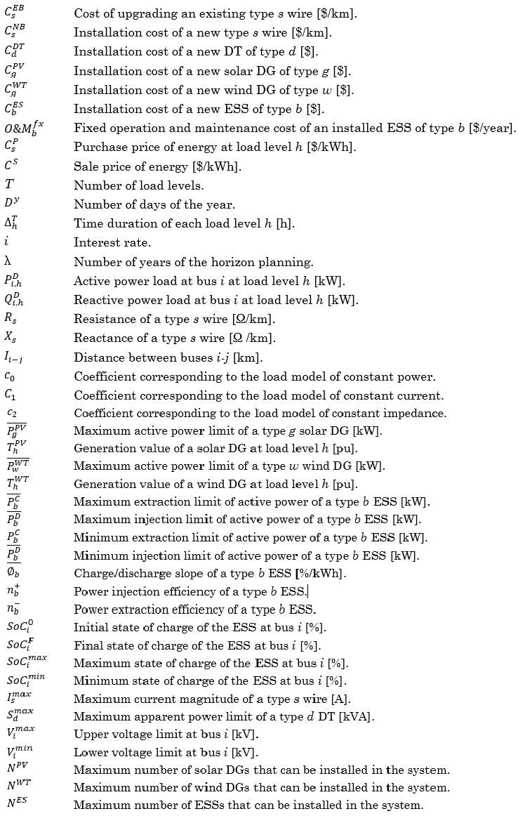
NOMENCLATURE

---

Parameters

Binary variables

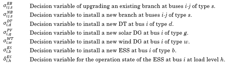
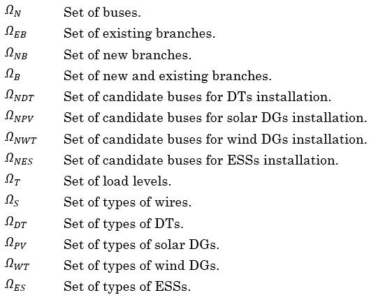
Continuous Variables

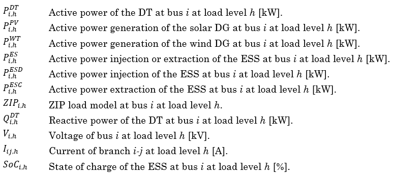
Sets

1. INTRODUCTION

---

The integration of distributed energy resources (DERs) in the electrical distribution systems recently became a customary strategy for distribution companies because it generates different benefits for them. The inclusion of DERs such as renewable DGs and ESSs improves some technical, operative, and economical problems in distribution systems and reduces environmental impacts on the planet. Therefore, several political and regulatory entities around the world encourage the integration of DERs in distribution systems [1]-[6].

In this context, Colombia encouraged the integration of DERs in electrical systems as a sustainable development goal by publishing different laws, rules, and regulations that establish a guideline for the operation and connection of DERs [7]-[9]. However, despite clear regulatory policies, these documents fail to establish a sequential strategy for distribution companies to operate and expand the electrical distribution systems considering the integration of DERs. Thus, distribution companies need to have reliable methodologies that integrate DERs in the operation and planning problems of distribution systems.

The specialized literature shows that some papers involve renewable DGs in the planning of low voltage (LV) networks [10]-[15]. Those papers considered the influence of solar DGs in the planning of LV networks but failed to consider the impact of wind DGs and the distribution companies as the owners of DGs. Moreover, only one paper considered the integration of solar DGs and ESSs in the planning of LV networks [16]. In that work, the distribution company owns the location and sizing problem of DTs. Unlike the above-mentioned works, this paper considers the distribution company as the owner of solar DGs, wind DGs, and ESSs, as well as the location and sizing problem of DTs in the expansion plans. Additionally, this paper also considers the optimal operation of ESSs for increasing the profit obtained from energy arbitrage.

The mathematical model proposed for planning the LV networks involving DERs is formulated as a mixed-integer non-linear programming problem (MINLP) and aims to minimize the fixed and operational costs of the LV distribution system and the total purchase cost of energy from the primary feeder. The fixed costs are associated with the investment cost of new elements (i.e., secondary branches, DTs, solar DGs, wind DGs, and ESSs), the upgrading cost of existing secondary circuits, and the operation and maintenance cost of new ESSs installed. The operational costs are associated with the present value of the technical energy losses costs in secondary circuits, DTs, and ESSs. Moreover, the profit obtained from energy arbitrage is also calculated in the present value.

The MINLP model is solved by using the Iterated Local Search (ILS) algorithm combined with a neighborhood scheme (i.e., branch exchange, upgrading of existing elements, and installation of new DTs and DERs). The choice of the ILS algorithm to solve the proposed model is due to the problem dimension, non-convexity, and binary nature of some variables as well as the computational complexity of the proposed NP-hard model. Also, the ILS metaheuristic has been used for solving problems with similar characteristics [17]-[19].

This paper is organized as follows. Section II outlines the mathematical formulation and describes the main aspects of the solution technique. Section III presents the results and discussion. Finally, Section IV provides commentary on the conclusions of this paper.

2. MATERIALS AND METHODS

---

2.1 Mathematical formulation

The MINLP model presented in (1) and (2) formulates the problem of the low voltage distribution system planning considering DERs. The nomenclature can be found at the beginning of this paper.

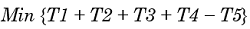
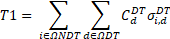
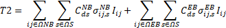
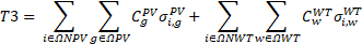
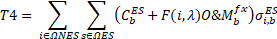
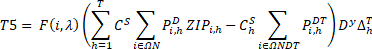
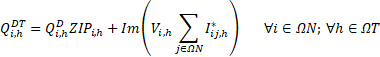
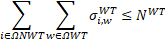
The five terms of the objective function (OF) of (1) are described in (3)-(7). The first term is the cost of installing new DTs. The term T2 is the cost of installing new secondary networks and of upgrading of the existing ones. The term T3 is the cost of installing new solar and wind DGs. The term T4 is the cost of installing new ESSs. Moreover, the term T4 also considers the fixed operation and maintenance cost (O&M) of new ESSs. Finally, the term T5 is the profit for energy arbitrage. Finally, the term T5 also considers the cost of the energy technical losses of secondary circuits, DTs, and ESSs. The annualized present value is calculated by the function F(i,λ)=(1-(1+ i) ^{- λ}) / i These five terms are described next.

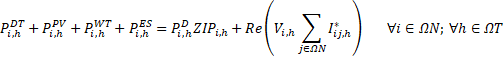
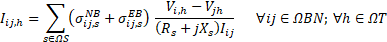
The set of constraints of (2) are explained next. Equations (8)-(9) are Kirchhoff’s laws represented by the active and reactive power nodal balance. Equation (10) calculates the currents flowing on the secondary circuits by using Ohm’s law. Equation (11) uses the ZIP model to represent the electrical demand.

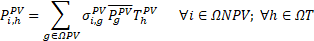
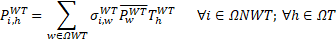
Equations (12)-(13) define the active power generated from the installed solar and wind DGs, respectively. Equations (14)-(20) model the operation of the installed ESSs, where δ_i,h^ESS represents the optimal operation of the ESSs. If δ_i,h^ESS=0, the ESS at node i is injecting power.

If δ_i,h^ESS=1, the ESS is extracting power. Equation (14) represents either the injecting or extracting power of the installed ESSs.

Equations (15)-(16) limit the charging and discharging power of the installed ESSs.

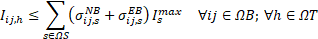
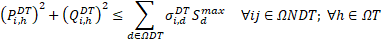
Equation (17) represents the state of charge of the installed ESSs. Equations (18)-(19) define the initial and final charge state of the installed ESSs. Equations (20)-(23) limit the charge state of the ESSs, the current in secondary circuits, the power in DTs, and the operation voltages of the system, respectively.

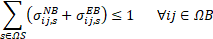
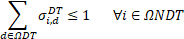
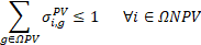
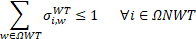
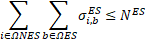
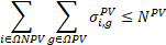
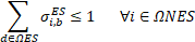
Equations (24)-(28) define that only one type of wire, DT, solar DG, wind DG, and ESS can be installed in one candidate node or branch. Finally, (29)-(31) restrict the number of solar DGs, wind DGs, and ESSs to install in the distribution systems.

2.2 Solution methodology

To solve the mathematical model described in (1)-(2), the ILS algorithm is used. This metaheuristic was proposed in [20] and it is used in this paper due to the dimension and complexity of (1)-(2). This algorithm performs an intensification and diversification process to find the global optimal solution, where the intensification process is performed by a local search through small changes in the current solution produced by using neighborhood schemes. The diversification process is conducted by perturbing the local optimum found in the local search to find a new initial solution for the next intensification process. Thus, the next local search can be executed in a new near area of the solution space, which allows the algorithm to find the global optimum and avoid being trapped in local optimums. The perturbation mechanism needs to be carefully controlled because weak perturbations could be insufficient in leaving local optimums and strong ones could be equivalent to random starts from different points in the solution space. The main aspects considered in the methodology are explained next.

2.2.1 Codification scheme

The low voltage system is encoded using a vector of integer numbers that represents the values of the decision variables. The information of the vector represents the size and location of the new and existing elements of the network (i.e., secondary circuits, DTs, renewable DGs, and ESSs). Each integer number is associated with the type of the installed element, and a zero value represents that no elements are installed.

2.2.2 Solution evaluation

The solutions generated by the neighborhood scheme are evaluated by using the two stage-decomposition method proposed in [21]. This easy-to-implement method finds the optimal operation of ESSs for minimizing the total purchase cost of energy and involves two stages. The first stage solves a linear programming (LP) model that temporarily removes electrical variables from the system and obtains the optimal ESSs operation from energy arbitrage. Then, in the second stage, the ESSs charge and discharge powers obtained from the first stage are treated as injections and consumptions of power (PQ nodes) in any power flow algorithm to obtain the real operating state of the system. The results obtained from this decomposition method are used for calculating the objective function and for verifying the feasibility of solutions. The LP model used to solve the operation problem of ESSs is described in [21]. The power flow algorithm used for solving the second stage of the decomposition method can be found in [22]. Also, if any of the mathematical model constraints are violated, the OF is penalized to ensure that only feasible solutions would be considered in the ILS algorithm.

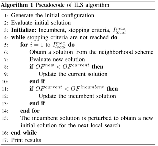
2.2.3 ILS Algorithm

The ILS algorithm uses an initial feasible solution to begin the first intensification process. The initial solution is generated from a constructive heuristic algorithm that connects all the loads of the secondary system to distribution transformers preserving the feasibility in the solution and the radial configuration topology of each secondary network.

When the initial solution is obtained, the local search is conducted by using a neighborhood scheme that executes small changes in the current solution, which accepts all evaluated solutions with low values of the objective function. The neighborhood scheme performs any of the following criteria: branch exchange, upgrade of the system existing elements, and installation of new DTs, solar DGs, wind DGs, and ESSs. The local search repeats itself until it achieves a predefined number of iterations. After the local search ends, the diversification process perturbs with major changes the best solution found in the intensification process.

The perturbation mechanism is carried out by applying the neighborhood scheme more than once. The ILS algorithm ends when the incumbent solution fails to improve for a predefined number of global iterations or when the ILS algorithm reaches a predefined maximum number of global iterations. The pseudocode of the ILS algorithm is described in Figure 1.

3. RESULTS AND DISCUSSION

---

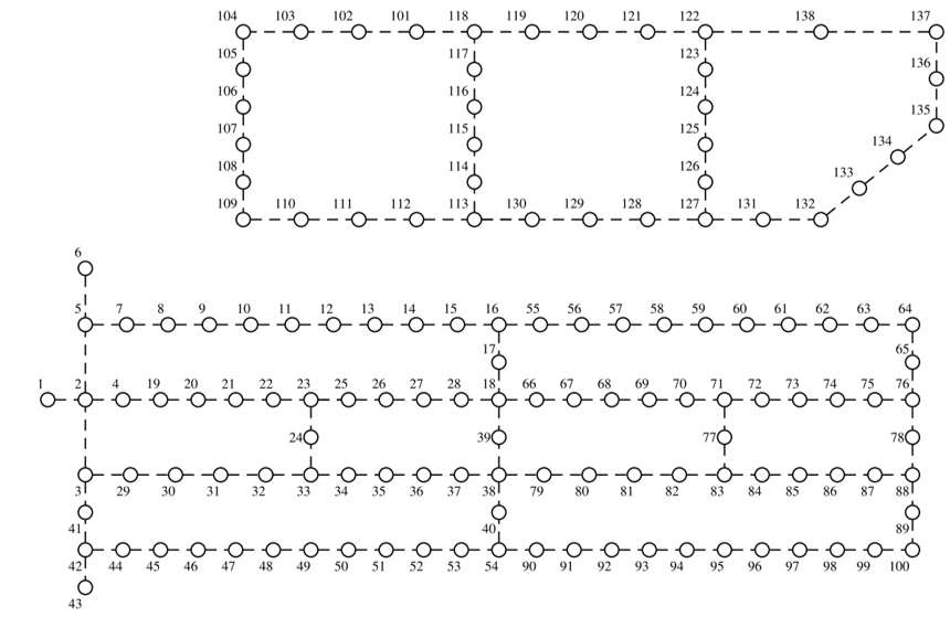
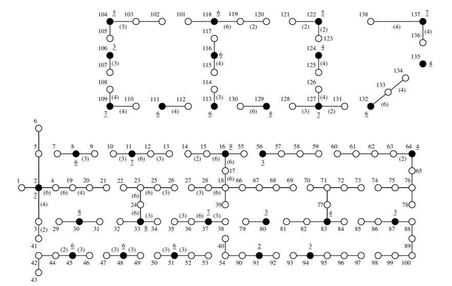
The methodology proposed in Section II is tested on an LV distribution system of 138 nodes to verify its effectiveness and robustness. Figure 2 shows the test system used, where the circles are load nodes and dashed lines are new branches. Figure 3 shows the daily curves of load demand, solar DGs, and wind DGs considered.

The nominal voltage of the system is 0.44 kV, the maximum voltage regulation is 10 %, and the values for base power and voltage are 300 kVA and 0.44 kV, respectively. The energy sale cost is 0.2 [USD/kWh], the interest rate is 10 %, the horizon planning is 20 years, and the ZIP load model coefficients c0 y c2 are 0.2 and 0.8, respectively.

The charge and discharge efficiencies, the deep of discharge, and the lifetime of the ESSs are 90 %, 100 % and 20 years, respectively. The lifetime of solar and wind DGs is 20 years, and the maximum number of elements that can be installed for solar DGs, wind DGs, and ESSs in the distribution system are 7, 5, and 6, respectively. Table 1 presents the energy purchase costs used. Moreover, it proposes the installation of 33 new DTs, 147 new secondary circuits, 15 new solar DGs, 14 new wind DGs, and 15 new ESSs (see Table 2). Full description and data of the test system used can be found in [23].

To validate the proposed methodology, two cases are compared: traditional expansion plans i) without DGs and ESSs (Case 1) and ii) with the installation of ESSs as well as solar and wind DGs (Case 2). The stopping criteria of the ILS algorithm stand at (i), for Case 1, 100 maximum global iterations or 35 global iterations if the incumbent solution fails improvement and (ii), for Case 2, 50 maximum global iterations or 15 global iterations without improvement. The maximum number of local iterations for Cases 1 and 2 are 100 and 800, respectively.

The proposed methodology was implemented using an interface between Matlab (2017b) and GAMS (24.5.4) in an Intel® Core i5-4460S 12 GB RAM PC. The solver CPLEX (version 12.6.2.0) was used to solve the LP model of the first stage of the decomposition method proposed in [18]. The CPU time for Cases 1 and 2 were 144.9 s and 7403.9 s, respectively. The present value of the obtained results is shown in Table 3, where the term TEL means technical energy losses. For Case 2, 6 ESSs (type 4) are installed in nodes 8, 11, 48, 109, 127, and 132; 7 solar DGs (type 4) in nodes 23, 38, 103, 110, 130, 131, and 136; 1 wind DG (type 3) in node 138; and 4 wind DGs (type 4) in nodes 19, 112, 119, and 130.

Figures 4 and 5 show the best configurations obtained for Cases 1 and 2, respectively, where the black circles are the locations of installed DTs. The numbers in parentheses in Figures 4 and 5 are associated with the type of wire installed for each secondary circuit; branches without a number are associated with type 1. Moreover, DT types are presented by an underlined number. Both cases obtained feasible solutions, and the branches downstream do not present a higher size of wire regarding secondary circuits upstream.

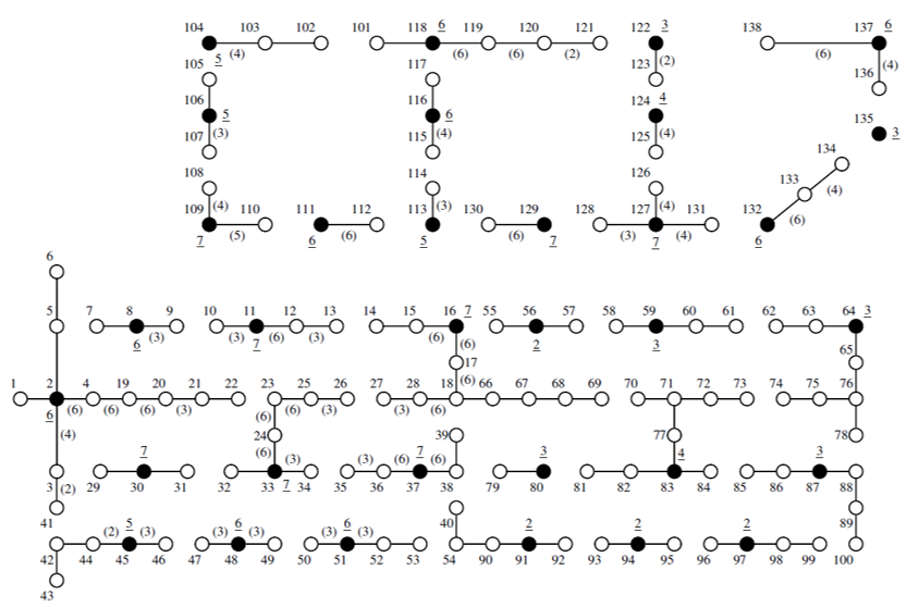
In Table 3, it is observed that Case 2 presents the highest value of the OF, which reflects an increase in profit from energy arbitrage due to the minimization of purchase cost. Also, it is observed the minimization of operational and fixed costs. The profit improved in Case 2 because the purchase cost is minimized by charging and discharging the installed ESSs with an optimal operation scheme based on the behavior of the energy prices and electrical demand. Moreover, the installation of new renewable DGs also minimizes the energy purchase cost.

The small difference in the sale cost between both cases stems from the ZIP model being used for demand (i.e., 20 % for constant power and 80 % for constant impedance). Case 2 has a bigger value in the installation of secondary circuits and a lower value in the installation of DTs regarding Case 1 because the installation of new DERs increases the sizes of wire in some branches and decreases the power capacity of some DTs. Furthermore, Case 1 has a lower total fixed cost (0.761) because Case 2 considers the installation of new DERs (8.089).

However, Case 2 has a lower total fixed cost when only the costs of secondary circuits and DTs are summed (0.738). Therefore, it is observed that the integration of new DERs in the distribution systems planning reduces the traditional fixed costs.

In Table 3, the higher total cost of TEL for Case 2 originates from the integration of new DERs in the networks that increase the magnitude of the currents flowing on some branches of the networks. Nevertheless, the increase in the total cost of TEL can be deemed insignificant due to the bigger benefits obtained from the minimization of the energy purchase cost. Moreover, the massive integration of DERs in networks with low nominal voltage values produces an increase in the TEL. Hence, it is advisable to consider the installation of DERs in the distribution systems planning of integrated primary and secondary networks to acquire a better distribution of power flows.

Figure 6 shows the total active power injected by the primary feeder for both cases. Case 1 does not consider the integration of DERs; thus, the total active power injected by the primary feeder for Case 1 has the same behavior of the demand curve of Figure 3. It can be observed in Figure 6 that the integration of DERs reduces the active power injected from the primary feeder that supplies the power of the LV networks connected to it. Figure 7 shows the sum of the injected and extracted power of the installed ESSs.

Figures 6 and 7 show how the installed ESSs are charged in hours of low demand and discharged in hours of peak demand. Thus, the power flows through DTs are decreased. It can be seen in Figures 3, 6, and 7 that the generated power in hours 12 and 13 nearly approaches zero because, during these hours, the solar DGs inject their maximum generated power, and the ESSs inject power at these hours. Moreover, the installation of new DERs decreased the peak power of the system at hour 20.

4. CONCLUSIONS

---

This paper proposed a new methodology to solve the problem related to the installation of DERs (i.e., renewable DGs and ESSs) in the distribution system planning problem of low voltage networks. The proposed methodology minimizes the fixed and operational costs of the networks and the total purchase cost of energy from the primary feeder. Hence, the total profit increased by minimizing the energy purchase cost of the system by installing new renewable DGs and ESSs. Moreover, the purchase cost is also minimized by way of an optimal operation of ESSs based on the behavior of energy prices and the electrical demand. The obtained results show that the integration of DERs in the distribution systems planning problem increases the profits of distribution companies from energy purchase and sale and it also reduces the fixed costs.

The total technical energy losses cost can increase with the integration of DERs because the profit obtained from the reduction of the purchase cost of demanded energy is more significant than the profit obtained from the minimization of the purchase cost of technical energy losses. Consequently, distribution companies can use the proposed methodology to measure the economical and operative advantages or disadvantages of the integration of DERs in the distribution systems planning problem of LV networks. The increase in technical energy losses can be controlled in the proposed methodology by adding a new constraint that limits the energy losses to a predefined value established by the distribution company.

Regarding the future work of this research, the uncertainty in renewable energy sources and electricity demand should be considered and involved in the model to have more realistic benefits.

5. ACKNOWLEDGMENTS

---

This work was funded by the Universidad Tecnológica de Pereira (Colombia) under Grant 6-22-4 and the Master’s in Electrical Engineering Program of the same University.

CONFLICTS OF INTEREST

---

The authors declare that there is no conflict of interest.

AUTHOR CONTRIBUTIONS

---

Alejandro Valencia-Díaz: participated in the conceptualization, methodology, software, results validation, and in the writing-review and editing process of the manuscript.

Ricardo A. Hincapié-Isaza: participated in the conceptualization, methodology, funding acquisition, and in the writing-review and editing process of the manuscript.

Ramón A. Gallego-Rendón: participated in the conceptualization, methodology, supervision, and in the reviewing process of the manuscript. All authors have read and agreed to the published version of the manuscript.

6. REFERENCES

---

• arrow_upward [1]   Ley 54/1997 del Sector Eléctrico, Jefatura del Estado de España, 1997. https://www.boe.es/eli/es/l/1997/11/27/54/con
• arrow_upward [2]   Acuerdo por el que se emite el Manual de Interconexión de Centrales de Generación con Capacidad Menor a 0.5 MW, Secretaría de Gobernación, México, 2016. http://www.dof.gob.mx/nota_detalle.php?codigo=5465576&fecha=15/12/2016
• arrow_upward [3]   Energy Networks Association, “Engineering Recommendation G98. Requirements for the Connection of Fully Type Tested Micro-Generators (up to and including 16 A per phase) in Parallel with Public Low Voltage Distribution Networks on or after 27 April 2019”, 2021. https://www.energynetworks.org/industry-hub/resource-library/erec-g98-requirements-for-connection-of-fully-type-tested-micro-generators.pdf
• arrow_upward [4]   Interconnection of On-Site Distributed Generation (DG), Public Utility Commission of Texas, Rule 25.211, 2017. https://www.puc.texas.gov/agency/rulesnlaws/subrules/electric/25.211/25.211ei.aspx
• arrow_upward [5]   Energy Networks Association, “Engineering Recommendation G99. Requirements for the Connection of Generation Equipment in Parallel with Public Distribution Networks, Energy Networks Association,” 2020. https://www.energynetworks.org/assets/images/Resource%20library/ENA_EREC_G99_Issue_1_Amendment_6_(2020).pdf
• arrow_upward [6]   Order Instituting Rulemaking to Modernize the Electric Grid for a High Distributed Energy Resources Future, California Public Utilities Commission (CPUC), 2021. https://docs.cpuc.ca.gov/PublishedDocs/Published/G000/M390/K664/390664433.PDF
• arrow_upward [7]   Ley 1715 de 2014, Integración de las Energías Renovables no Convencionales al Sistema Energético Nacional, Congreso de Colombia. Colombia, 2014. http://www.upme.gov.co/Normatividad/Nacional/2014/LEY_1715_2014.pdf
• arrow_upward [8]   Comisión de Regulación de Energía y Gas, “Resolución No 030 de 2018 (26 de febrero de 2018)”, Colombia, 2018. http://apolo.creg.gov.co/Publicac.nsf/
• arrow_upward [9]   Comisión de Regulación de Energía y Gas, “Resolución No 002 de 2021 (7 de enero de 2021)”, Colombia, 2021. http://apolo.creg.gov.co/Publicac.nsf/1c09d18d2d5ffb5b05256eee00709c02/8e71dd926eb1d0dc0525866a005921dc/$FILE/Creg002-2021.pdf
• arrow_upward [10] J. E. Mendoza; M. E. López; S. C. Fingerhuth; H. E. Peña; C. A. Salinas, “Low Voltage Distribution Planning Considering Micro Distributed Generation”, Electr. Power Syst. Res., vol. 103, pp. 233-240, Oct. 2013. https://doi.org/10.1016/j.epsr.2013.05.020
• arrow_upward [11] L. Verheggen; R. Ferdinand; A. Moser, “Planning of Low Voltage Networks Considering Distributed Generation and Geographical Constraints”, in IEEE International Energy Conference, Leuven, 2016, pp. 1-6
• arrow_upward [12] A. Hadjsaid; V. Debusschere; M-C. Alvarez-Herault; R. Caire, “Considering Local Photovoltaic Production in Planning Studies for Low Voltage Distribution Grids”, in IEEE Milan PowerTech, Milano, 2019, pp. 1-5. https://doi.org/10.1109/PTC.2019.8810613
• arrow_upward [13] J. Jiménez; J. E. Cardona; S. X. Carvajal, “Location and optimal sizing of photovoltaic sources in an isolated mini-grid”, TecnoLógicas, vol. 22, no. 44, pp. 61-80, Jan. 2019. https://doi.org/10.22430/22565337.1182
• arrow_upward [14] L. F. Gaitán; J. D. Gómez; E. Rivas-Trujillo, “Análisis Cuasi-Dinámico de un sistema de distribución local con generación distribuida. Caso de estudio: Sistema IEEE 13 Nodos”, TecnoLógicas, vol. 22, no. 46, pp. 195-212, Sep. 2019. https://doi.org/10.22430/22565337.1489
• arrow_upward [15] K. Kasturi; C. Kumar Nayak; S. Patnaik; M. Ranjan Nayak, “Strategic integration of photovoltaic, battery energy storage and switchable capacitor for multi-objective optimization of low voltage electricity grid: Assessing grid benefits”, Renew. Energy Focus, vol. 41, pp. 104-117, Jun. 2022. https://doi.org/10.1016/j.ref.2022.02.006
• arrow_upward [16] V. Vai; M.-C. Alvarez-Herault; B. Raison; L. Bun, “Optimal Low-voltage Distribution Topology with Integration of PV and Storage for Rural Electrification in Developing Countries: A Case Study of Cambodia”, J. Mod. Power Syst. Clean Energy, vol. 8, no. 3, pp. 531-539, May 2020. https://doi.org/10.35833/MPCE.2019.000141
• arrow_upward [17] M. Moreira de Souza; P. H. González; L. Satoru Ochi; S. Martins, “A Hybrid Iterated Local Search Heuristic for the Traveling Salesperson Problem with Hotel Selection”, Comput. Oper. Res., vol. 129, pp. 1-16, Jan. 2021. https://doi.org/10.1016/j.cor.2021.105229
• arrow_upward [18] D. Calmels, “An Iterated Local Search Procedure for the Job Sequencing and Tool Switching Problem with Non-Identical Parallel Machines”, Eur. J. Oper. Res., vol. 297, no. 1, pp. 66-85, May. 2021. https://doi.org/10.1016/j.ejor.2021.05.005
• arrow_upward [19] M. Alicastro; D. Ferone; P. Festa; S. Fugaro; T. Pastore, “A Reinforcement Learning Iterated Local Search for Makespan Minimization in Additive Manufacturing Machine Scheduling Problems”, Comput. Oper. Res., vol. 131, pp. 1-14, Jul. 2021. https://doi.org/10.1016/j.cor.2021.105272
• arrow_upward [20] H. R. Lourenço; O. C. Martin; T. Stützle, “Iterated Local Search”, in Handbook of Metaheuristics, First Edition, USA: Springer, 2003, pp. 320-353. https://doi.org/10.1007/b101874
• arrow_upward [21] A. Valencia; R. A. Hincapié; R. A. Gallego, “Optimal Location, Selection, and Operation of Battery Energy Storage Systems and Renewable Distributed Generation in Medium–Low Voltage Distribution Networks”, J. Energy Storage., vol. 34, pp. 1-16, Feb. 2021. https://doi.org/10.1016/j.est.2020.102158
• arrow_upward [22] R. D. Zimmerman; C. E. Murillo-Sánchez (2020). MATPOWER. User’s Manual: Version 7.1 [Software]. https://matpower.org
• arrow_upward [23] A. Valencia; R. A. Hincapié; R. A. Gallego, “Database of the distribution test system”. [Online]. http://academia.utp.edu.co/planeamiento/files/2021/06/138N-TestSystem.pdf