Sensitivity Analysis and Small-Signal Stability of Grid Following Converters

Received: April 6, 2022
Accepted: June 6, 2022
Available: July 1, 2022

How to cite / Cómo citar
S. Sepúlveda-García; A. Garcés-Ruíz, “Sensitivity Analysis and Small-Signal Stability of Grid Following Converters,” TecnoLógicas, vol. 25, nro. 54, e2383, 2022. https://doi.org/10.22430/22565337.2383

Abstract

This article presents a small-signal study, based on a sensitivity analysis, of a voltage source converter (VSC) operating as a grid-following device. This type of operation is standard for integrating distributed energy resources directly into a primary grid without considering the control over specific variables (e.g., voltage and frequency), thus maximizing the amount of injected active power. The present study adopted the classical vector-oriented control based on the linearization method of the averaged model; hence, this analysis is limited to linear controls. The main objective of this study is to evaluate how each controller parameter influences the system’s stability. To conduct the sensitivity analysis, an averaged model in the dq reference frame of the VSC was employed to describe the system dynamics in the equivalent state-space model. Afterward, the stability was analyzed through a sensitivity analysis of the eigenvalues of the corresponding state matrix. The numerical results demonstrate that the main problems for the stability of VSCs operating as grid-following converters are threefold: a high value of the filter inductance, a non-ideal impedance that appears depending on the connection point, and poor coordination of the parameters of the Kp controllers. These results are compared to a simple bifurcation analysis of the state matrix, which consists of a diagram that describes the variation in eigenvalues when a parameter changes, thus proving their validity.

Keywords: Grid-following converters, Hopf bifurcation, Sensitivity analysis, Vector-oriented control, Voltage source converter.

Resumen

El presente artículo presenta un estudio de pequeña señal, basado en el análisis de sensibilidad, del convertidor Voltage Source Converter (VSC) operando como dispositivo de seguimiento de red. Este tipo de operación es común para la integración de recursos energéticos distribuidos directamente a la red primaria sin considerar el control sobre variables específicas como la tensión o la frecuencia, maximizando así la cantidad de potencia activa inyectada. El presente estudio adopta el clásico Control Vectorial Orientado basado en la linealización del modelo promediado, por tanto, este análisis es limitado a controles lineales. El objetivo principal de esta investigación consistió en evaluar cómo influye cada parámetro del controlador en la estabilidad del sistema. Con el fin de realizar el análisis de sensibilidad, se empleó un modelo medio en el marco de referencia dq del VSC para describir la dinámica del sistema en el espacio de estados equivalentes; posteriormente, se buscó la estabilidad mediante un análisis de sensibilidad de los valores propios de la matriz de estado correspondiente, cuyos resultados numéricos demostraron que los principales problemas para la estabilidad de los VSC que operan como convertidores de seguimiento son tres: un valor elevado de la inductancia del filtro, la presencia de una impedancia no ideal que aparece en función del punto de conexión, y una mala coordinación de los parámetros de los controladores Kp. Estos resultados se han comparado con un simple análisis de bifurcación de la matriz de estado, que consiste en un gráfico que describe el movimiento de los valores propios cuando cambia un parámetro, corroborando así su validez.

Palabras clave: Convertidores seguidores de red, Bifurcación tipo Hopf, Análisis de sensibilidad, Control vectorial orientado, Convertidor de fuente de tensión.

1. INTRODUCTION

Power electronic converters are key elements in the modern electrical grid, they are immerse from applications of High Voltage Direct Current applications (HVDC) [1] to Low Voltage Direct Current (LVDC) [2], [3] applications. Moreover, the penetration of Distributed Energy Resources (DERs) into the grids make a strongly dependence of this devices [4].

Those DERs usually operate in DC, and hence requires a converter, named Voltage Source Converter (VSC), to integrate the renewable resource into the primary grid [5]. Although this is a relatively new technology in Colombia, grid operators have an increasing interest in studying the impact of these devices on the power distribution grid. There is a consensus in the necessity of diversify the generation matrix, and increase the penetration of DERs into the grid which naturally lead to an increase in the presence of VSCs [6]. The international community identified that the stability analysis of inverter-based systems is a fundamental challenge for the massive integration of renewable energy in the near future, as demonstrated in the most recent document of the IEEE-PES Task Force on Microgrid Stability Definitions, Analysis, and Modeling [7].

Power electronic converters introduce new dynamic phenomena compared to conventional power systems dominated by the dynamic behavior of synchronous machines. The issues related to the stability of these new grids are described in [7], [8], where it is clear that the control of the converter is a fundamental element in the study of small-signal stability [9].

The classical vector-oriented control employed for electrical machines has been adapted to be applicable in power electronic converters and nowadays is one of the most commercial [10], [11]. This control has several loops that interact together, generating complex dynamics, however, in order to simplify the analysis, some studies make an approximation by analyzing the average model of the VSC, which only takes into account the dynamic response and not the complete model which includes the switch losses [9].

Several studies have been conducted to analyze the stability of the voltage source converter, such as the unstable phenomenon in the three-phase case [12]. Furthermore, it has been reported that one of the main problems affecting the small-signal stability of the VSC system is the influence of a non-ideal grid in the system [13]–[15]. This study has different approaches for the analysis of the stability. In [16], [17] it was analyzed directly in the Nonlinear equivalent; however, this approach is not suitable for large systems. The passivity theory is used in [18] in order to study the small-signal stability of the VSC. A recent approach made use of the Graph theory together with the state space [19], this approach demonstrates to be more robust and faster than the studies previously described.

However, it is still preferred to use linearization methods due to its simplicity to calculate the instability [20]. Recently there has also been an interest in stability analysis of the single-phase converter due to its wide applications in electrical systems [14], [21].

Nevertheless, sensitivity analysis is rarely discussed for these converters, despite its usefulness in determining the elements and parameters of the system that cause the most problems to the stability in a numerical way [22]. Therefore, this article aims to fill this gap, showing a sensitivity analysis for the VSC and determining how the parameters affect the system's stability. The stability analysis of inverter-based power systems is classified into control-system stability and power supply balance stability [23] The former is divided into the electric machine and converter stability, whereas the latter is divided into voltage and frequency stability. The study presented here devises the converter stability, although it also concerns voltage stability on the dc-link, both from the small-signal perspective. As mentioned before this approach is limited to controllers based on average models, other controllers such as the Sliding Mode control are more robust, however some industrial applications still make use of PIs controllers in cascade with the simplified average models due to its ease implementation [24].

The rest of the paper is organized as follows: First, the converter model is described mathematically in Section II. Next, in Section III, the mathematical model is linearized around the operating point. Finally, in Section IV, a sensitivity analysis of the system's elements is performed. Conclusions are presented in Section V, followed by a brief list of references. This article was previously introduced at the international conference X-Sicel.

2. METHODOLOGICAL ASPECTS

2.1 Model of the VSC

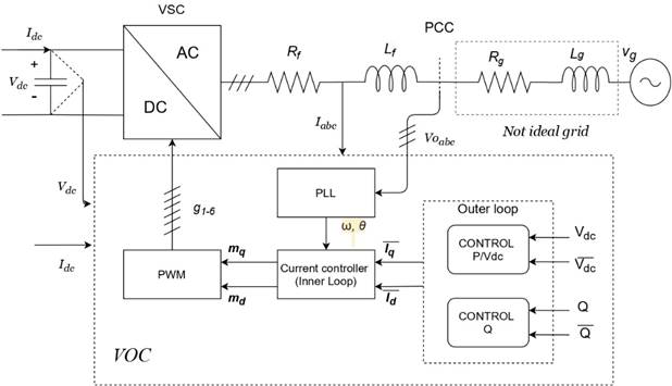
The employed model of the VSC is a simplified model with an ideal grid and switching losses close to zero, this approximation is known as average model, and provides a fair estimation of the stability of the VSC; for more robust or detailed applications it is necessary to make use of different type of controllers. The model is continuous with a modulation index m_i ∈ [-1,1]. The control to be studied is the conventional vector-oriented control, the most common approach in commercial converters. The circuit, together with its control, is described in Figure 1 [25].

Figure 1. Voltage source converter (VSC) with vector-oriented control (VOC). Source: Created by the authors.

2.1.1 Model of the grid

Kirchhoff’s second law is applied to the loop comprised of the converter output, the filter, and the point of common coupling (PCC), as given in (1) and (2).

(1)

(2)

All variables are evident from the figure above. Note that the system is described in the dq frame because the variables are easier to control by PI-type controllers in a stationary frame of reference than in a rotating one. Similarly, the relationship for the non-ideal grid is given in (3) and (4).

(3)

(4)

From the set of equations described above, it is possible to demonstrate that the tensions in the point of common coupling are (5) and (6), respectively.

(5)

(6)

Furthermore, it is possible to demonstrate that the dynamics of the currents in the ac side in the dq frame are (7) and (8).

(7)

(8)

The set of equations describing the system's dynamics is completed with the voltage dynamics at the DC side (9). This voltage can be obtained through the power balance as follows.

(9)

The vector-oriented control has a structure with different modules named phase-locked-loop (PLL), inner-loop, and outer-loop. Each of these modules is briefly described below.

2.1.2 Phase-Locked-Loop (PLL)

The phase-locked-loop is in charge of coordinating the converter with the pre-existing network; the block diagram is described in Figure 2 .

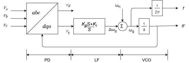
Figure 2. Phase Locked Loop (PLL). Source: Created by the authors.

By defining an auxiliary variable γ_pll. The model can be mathematically rewritten at the PI controller's output [26], as shown in (10) and (11).

(10)

(11)

2.1.3 Inner Loop

The inner loop controls the currents of the converter on the AC side; the block diagram is shown in Figure 3.

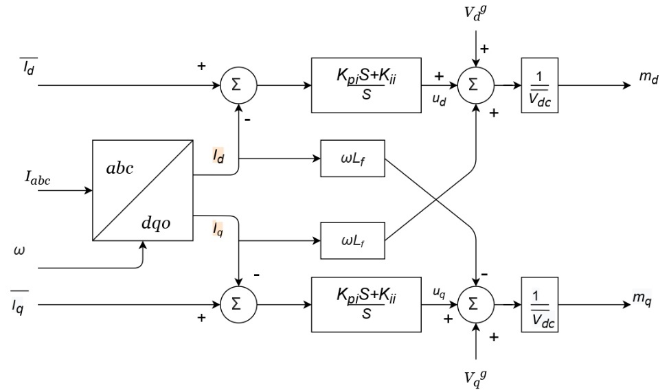
Figure 3. Inner Loop. Source: Created by the authors.

Similarly, a set of auxiliary variables γ_d and γ_q are defined to describe the model mathematically as (12)-(15).

(12)

(13)

(14)

(15)

The variables with a bar, such as x ̅ are references. Equations (5) and (6) are replaced into (10) and (11), so it is possible to obtain (16) and (17).

(16)

(17)

That represents the control variables of the system.

2.1.4 Outer loop

Finally, the outer loop is in charge of controlling the DC voltage of the system; the block diagram is described in Figure 4.

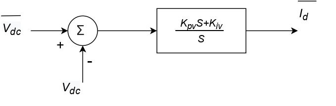
Figure 4. Outer Loop. Source: Created by the authors.

Which can be described as (18)-(19).

(18)

(19)

Since the unitary power factor is assumed, there is no control over reactive power.

2.2 State-Space Model

Equations (7) and (19) are collected. Observe that the state variables are x=[i_d, i_q, v_dc, γ_d, γ_q, γ_v ]^T, the control variables y=[v_d^s, v_q^s ]^T, and the input variables u=[v_d^g, v_dc, I_dc, i_q*]^T. Note that the variables θ' and γ_pll are not considered since, in this representation, there are no control and system state variables in the PLL model and vice versa; therefore, the frequency is supposed to be ideal. These equations follow the form described in (20) and (21).

(20)

(21)

The aim is to obtain a system of linear equations like (22), which may be linearized around the equilibrium point, using the expressions described in (23) and (24) [27].

(22)

(23)

(24)

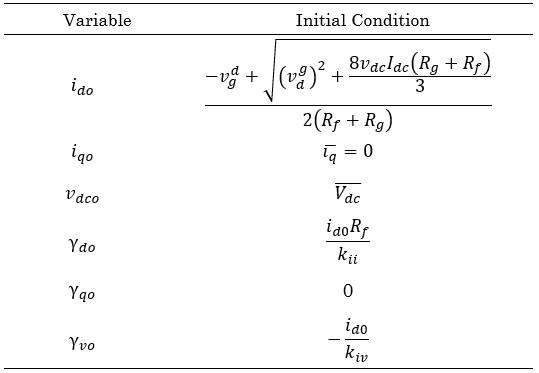
The system's initial conditions can be obtained by considering stable operation (i.e., the dynamics are zero; therefore, the derivatives are equal to zero), these values are given in Table 1.

Table 1. Initial conditions
Source: Created by the authors.

The results of the linearization around the operating point are given by (25), where the elements J₃ of the third row are given by (26)-(31).

(25)

(26)

(27)

(28)

(29)

(30)

(31)

2.2.1 Sensitivity Analysis

The sensitive analysis aims to determine the influence of each element of the state matrix on the system's eigenvalues. That is to say, to evaluate how a change in the value of one component could affect the position of the eigenvalues. The participation factor p_i expresses this relation which indicates the rate of change of a specific eigenvalue against an element of the state matrix as shown in (32).

(32)

Where a_km corresponds to the entry in row k, with column m; φ_i corresponds to the eigenvectors on the left and ϕ_i to the eigenvectors on the right. Notice that (25) exposes the variation of the eigenvalue λ_i concerning the element a_km; likewise, it is possible to observe that the final result is a three-dimensional matrix, known as a tensor.

It is difficult to visualize the results in a tensor. Therefore, the influence of a specific parameter (e.g., the inductance), immersed in different elements of the state matrix, is obtained by applying the chain rule in (32) , resulting in (33).

(33)

Where x corresponds to the parameter whose influence on the oscillation mode i is to be known, finally, it is necessary to clarify that the numerical value obtained from the participation factors does not have much relevance. However, their relative value does. It is taken to measure how much a variation affects or not one or another oscillation mode.

3. RESULTS AND DISCUSSION

The stability analysis was performed in a realistic system with system parameters and constants shown in Tables (2) and (3), respectively.

Table 2. System Parameters
Source: Created by the authors.

Parameter	Value
Capacitance (C)	2200 μF
Filter inductance (L_f)	55 mF
Filter Resistance (R_f)	50 mΩ
Source inductance (L_g)	10 mH
Source Resistance (R_g)	20 mΩ
Source voltage (v_d^g)	380 V
DC voltage (v_dc)	1000 V
DC current (I_dc)	2 A

Table 3. Control Parameters
Source: Created by the authors.

Parameter	Value
k_pi	29.33
k_pv	1.1729
k_ii	7106
k_iv	312.66

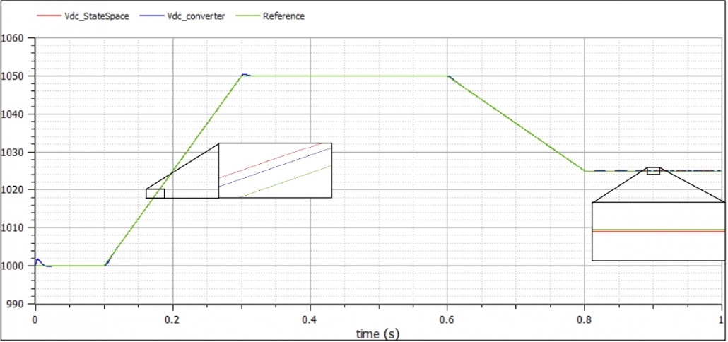
The model was implemented in OpenModelica and was compared with the linearization around the operation point, proving a good approximation, as depicted in Figure 5. Note that it is not strictly necessary to use per unit variables.

Figure 5. Comparison between the statespace model and the complete model. Source: Created by the authors.

The system's stability can be analyzed by positioning the eigenvalues of the state matrix as mentioned in (34).

(34)

For the base case, they take the value described in (35).

(35)

This equation assumes that the system operates in steady-state; however, we want to answer the question: how do the system parameters affect the system's stability?

This question can be solved in the first instance by applying (25) where the generic case (i.e., a three-dimensional matrix) is obtained; however, visualizing the results is somewhat complex. With the help of (26), it is possible to get more visible results. Note that each numerical value in Table 4 and Table 5 indicates the rate of change of the eigenvalue concerning the system parameter.

Table 4. Participation factors (real part) system parameters
Source: Created by the authors.

Parameter	L_f	C
p₁	3796.68	-4171.90
p₂	3796.68	-4171.90
p₃	1057.86	2245.72
p₄	1057.86	2245.72
p₅	4854.54	-1.14 × 10-27
p₆	4854.54	-1.14 × 10-27

Table 5. Participation factors (real part) control parameters
Source: Created by the authors.

Parameter	k_pi	k_pv	k_ii	k_iv
p₁	-6.83	-91.424	-0.0035	0.371
p₂	-6.83	-91.424	-0.0035	0.371
p₃	-3.65	56.75	0.0035	-0.37
p₄	-3.65	56.75	0.0035	-0.37
p₅	-9.09	3.92 × 10-30	-1.911 × 10-19	-3.49 × 10-32
p₆	-9.09	3.92 × 10-30	-1.911 × 10-19	-3.49 × 10-32

As can be deduced, the participation factors, like the eigenvalues, come in conjugate pairs. As mentioned, their numerical value does not have that much impact; what matters are the associated relative values (as well as their sign). It is possible to deduce, for example, that a slight change in the inductance value will noticeably affect the positioning of all the eigenvalues (especially λ_1,2,5,6), reducing the stability margins. While in the case of an increase in the capacitance value, the stability margin of the eigenvalues λ_1,2 is increased at the cost of a reduction in the margins of the eigenvalues λ_4,5.

Contrary to the case of the inductance, an increase in the constant k_pi will increase the stability margins of the system; it is also noticeable how the real part of the eigenvalues λ_5,6 is only influenced by the system's inductance and the current controller's proportional action.

It is also remarkable how the increase of the other constants can improve and worsen the positioning of some eigenvalues.

Similarly, the imaginary part of the eigenvalues is essential since they affect the so-called damping ratios described in (36). A value lower than 10% of these damping ratios affects the system, and control processes must be developed to increase them.

(36)

Hence it is worth asking, how do changes in controller parameters and constants affect the imaginary part? The answer to this question may be obtained from Tables 6 and 7.

Table 6. Participation factors (imaginary part) system parameters
Source: Created by the authors.

Parameter	Lf	C
p₁	-690.37	-96230.6
p₂	690.37	96230.6
p₃	-777.58	22583.16
p₄	777.58	-22583.16
p₅	16.01	3.44×10^-27
p₆	-16.01	-3.44×10^-27

Table 7. Participation factors (imaginary part) control parameters
Source: Created by the authors.

Parameter	k_pi	k_pv	k_ii	k_iv
p₁	0.26	149.74	0.018	0.115
p₂	-0.26	−149.74	-0.018	-0.115
p₃	−3.14	−72.74	0.013	0.113
p₄	3.14	72.74	-0.013	-0.113
p₅	−8.92	3.86×10^-30	0.033	-2.20×10^-32
p₆	8.92	-3.86×10^-30	-0.033	2.20×10^-32

As aforementioned, eigenvalues come in conjugate pairs, indicating that a change in each parameter will move the eigenvalues closer to (or further away from) the real axis depending on the case. For example, an increase in k_pi is accompanied by an increase in the damping ratios of the system. Whereas for k_ii an increase moves the eigenvalues away from the real axis, implying that the damping ratios decrease significantly.

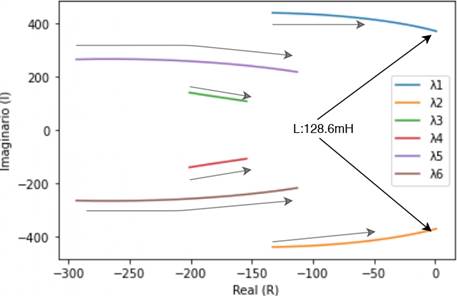
These results described above can be easily verified through a simple bifurcation analysis, where (34) is used, and a given parameter is varied, plotting the path of the eigenvalues as shown in Figure 6 and Figure 7.

Figure 6. Bifurcation of the system for L 50150 mH . Source: Created by the authors.

Figure 7. Bifurcation of the system for kii [5-100]×103. Source: Created by the authors.

As predicted from the analysis of the participation factors, an increase in the inductance value reduces the stability margin until a Hopf bifurcation occurs. Moreover, increasing the integral action of current control increases damping ratios. Consequently, the eigenvalues λ_5,6moves away from the real axis.

Finally, it is interesting to know what happens when a non-ideal network is in the system. In this scenario, the participation factors described in Table 8 are presented.

Table 8. Participation factors (real part) system parameters
Source: Created by the authors.

Parameter	L_f	L_g
p_1,2	3947.41±288.29	475.8±55.07
p_3,4	1180.67±686.03	161.97±84.83
p_5,6	4856.19±509.26	-3.27×10^-30±6.66×10^-31

As can be seen, these indicate that with the presence of the non-ideal inductance, the stability margins of the first four eigenvalues are reduced. In addition, it can be noticed how it slightly changes the participation factors of the inductance L., becoming more "sensitive" to changes, which happens with the other parameters of the network and control. Therefore, the presence of a non-ideal network significantly affects the system's stability, reducing the stability margins and making the system more sensitive to changes in other parameters.

4. CONCLUSIONS

In this paper, a sensitivity analysis is used to determine numerically how system parameters and controller constants influence the stability of a VSC operating as a grid feeder. As remarked, this analysis can be helpful since it can easily detect the parameters that cause stability problems, the proposed approach is based in the average model neglecting the losses in the grid and the switch losses. In the same way, these variables are suitable to control to improve the positions of some eigenvalues, increase margins of stability, damping ratios, or simply design the converter to maintain stability when they are fixed variables As may be deduced from the results, an increase in the proportional action of the current controller increases the stability margins of all the eigenvalues, which is helpful since it can be coordinated with a high inductance (or capacitance) value for filtering, which notoriously these margins. From the perspective of the control, it is desired to have a high value for the integral action since it ensures zero steady-state error; nevertheless, as can be deduced from the analysis, a high value of this parameter reduce significantly the damping ratios of the system, hence, a study of the control and design of the VSC must be done with a corresponding study of stability. For future works, it is recommended to include more detailed models of the power source and if necessary, the incorporation of DC-DC converter in the model. In addition, it is important to analyze the influence of the R/X ratio in the case of microgrids; furthermore, the sensitivity analysis can be used in a general way in the study of stability of any electrical system that could be represented as its equivalent state-space model, for this reason it is recommended to make a sensitivity analysis of a modern controllers such as the Non-Linears widely proposed in the technical literature.

5. ACKNOWLEDGMENTS

This paper is a result of project Integra2023, code 111085271060, contract 80740-774-2020, funded by the Ministry of Science, Technology, and Innovation (Minciencias) and developed by the ICE3 Research Group at Universidad Tecnológica de Pereira (UTP).

CONFLICTS OF INTEREST

The authors have no conflicts of interest to declare. All co-authors have seen and agree with the manuscript's contents, and there is no additional financial interest to report, different from Minciencias and Universidad Tecnológica de Pereira. We certify that the submission is original work and is not under review at any other publication.

AUTHOR CONTRIBUTIONS

Simón Sepúlveda-García: Methodology, Implementation, Writing.

Alejandro Garcés-Ruíz: Conceptualization, Methodology, Writing, Validation.

6. REFERENCES

[1] A. Kalair; N. Abas; N. Khan, “Comparative study of HVAC and HVDC transmission systems”, Renew. Sust. Energ. Rev., vol. 59, pp. 1653–1675, Jun2016. https://doi.org/10.1016/j.rser.2015.12.288
[2] A. Garces, “Uniqueness of the power flow solutions in low voltage direct current grids”, Electr. Power Syst. Res., vol. 151, pp. 149–153, Oct. 2017. https://doi.org/10.1016/j.epsr.2017.05.031
[3] A. Garcés-Ruiz, “Small-signal stability analysis of dc microgrids considering electric vehicles”, Rev. Fac. de Ing., no. 89, pp. 52-58, Oct. 2018. https://doi.org/10.17533/udea.redin.n89a07
[4] C. García-Ceballos; S. Pérez-Londoño; J. Mora-Flórez, “Integration of distributed energy resource models in the VSC control for microgrid applications”, Electr. Power Syst. Res., vol. 196, p. 107278, Jul. 2021. https://doi.org/10.1016/j.epsr.2021.107278
[5] T. Dragičević; S. Vazquez; P. Wheeler, “Advanced Control Methods for Power Converters in DG Systems and Microgrids”, IEEE Trans. Ind. Electron., vol. 68, no. 7, pp. 5847–5862, Jul. 2021. https://doi.org/10.1109/TIE.2020.2994857
[6] D. López-García; A. Arango-Manrique; S. X. Carvajal-Quintero, “Integration of distributed energy resources in isolated microgrids: the Colombian paradigm”, TecnoLógicas, vol. 21, no. 42, pp. 13–30, May 2018. https://doi.org/10.22430/22565337.774
[7] Z. Shuai et al., “Microgrid stability: Classification and a review,” Renew. Sust. Energ. Rev., vol. 58, pp. 167–179, May. 2016. https://doi.org/10.1016/j.rser.2015.12.201
[8] M. Farrokhabadi et al., “Microgrid Stability Definitions, Analysis, and Examples”, IEEE Trans. Power Syst., vol. 35, no. 1, pp. 13–29, Jan. 2020. https://doi.org/10.1109/TPWRS.2019.2925703
[9] W. Du; Q. Fu; X. Wang; H. F. Wang, “Small-signal stability analysis of integrated VSC-based DC/AC power systems – A review”, Int. J. Electr. Power Energy Syst., vol. 103. pp. 545–552, Dec. 2018. https://doi.org/10.1016/j.ijepes.2018.06.015
[10] T. Kalitjuka, “Control of Voltage Source Converters for Power System Applications”, (M.S. thesis), Department of Electric Power Engineering, Norwegian University of Science and Technology, Trondheim, 2011. https://ntnuopen.ntnu.no/ntnu-xmlui/handle/11250/257163?show=full
[11] J. Rocabert; A. Luna; F. Blaabjerg; P. Rodríguez, “Control of power converters in AC microgrids”, IEEE Trans. Power Electron., vol. 27, no. 11, pp. 4734–4749, Nov. 2012. https://doi.org/10.1109/TPEL.2012.2199334
[12] M. Huang; Y. Peng; C. K. Tse; Y. Liu; J. Sun; X. Zha, “Bifurcation and Large-Signal Stability Analysis of Three-Phase Voltage Source Converter under Grid Voltage Dips”, IEEE Trans. Power Electron., vol. 32, no. 11, pp. 8868–8879, 2017. https://doi.org/10.1109/TPEL.2017.2648119
[13] M. Huang; C. K. Tse; S. C. Wong; C. Wan; X. Ruan, “Low-frequency hopf bifurcation and its effects on stability margin in three-phase PFC power supplies connected to non-ideal power grid”, IEEE Trans. Power Electron., vol. 60, no. 12, pp. 3328–3340, Dec. 2013. https://doi.org/10.1109/TCSI.2013.2264698
[14] H. Chen; W. Yu; Z. Liu; Q. Yan; I. Adamu Tasiu; Z. Han, “Low-Frequency Instability Induced by Hopf Bifurcation in a Single-Phase Converter Connected to Non-Ideal Power Grid”, IEEE Access, vol. 8, pp. 62871–62882, 2020. https://doi.org/10.1109/ACCESS.2020.2983479
[15] S. Rezaee; A. Radwan; M. Moallem; J. Wang, “Voltage source converters connected to very weak grids: Accurate dynamic modeling, small-signal analysis, and stability improvement”, IEEE Access, vol. 8, pp. 201120–201133, 2020. https://doi.org/10.1109/ACCESS.2020.3035840
[16] Z. Yang; R. Ma; S. Cheng; M. Zhan, “Nonlinear Modeling and Analysis of Grid-Connected Voltage-Source Converters under Voltage Dips”, IEEE Trans. Emerg. Sel. Topics Power Electron., vol. 8, no. 4, pp. 3281–3292, Dec. 2020. https://doi.org/10.1109/JESTPE.2020.2965721
[17] K. F. Krommydas; A. T. Alexandridis, “Nonlinear Analysis Methods Applied on Grid-Connected Photovoltaic Systems Driven by Power Electronic Converters”, IEEE Trans. Emerg. Sel. Topics Power Electron., vol. 8, no. 4, pp. 3293–3306, Dec. 2020. https://doi.org/10.1109/JESTPE.2020.2992969
[18] L. Harnefors; X. Wang; A. G. Yepes; F. Blaabjerg, “Passivity-Based Stability Assessment of Grid-Connected VSCs-An Overview”, IEEE Trans. Emerg. Sel. Topics Power Electron., vol. 4, no. 1, pp. 116–125, Mar. 2016. https://doi.org/10.1109/JESTPE.2015.2490549
[19] Q. Geng; X. Zhou, “Small signal stability analysis of VSC based DC systems using graph theory”, Int. J. Electr. Power Energy Syst., vol. 137, p. 107830, May. 2022. https://doi.org/10.1016/j.ijepes.2021.107830
[20] R. Yin et al., “Modeling and stability analysis of grid-tied VSC considering the impact of voltage feed-forward”, Int. J. Electr. Power Energy Syst., vol. 135, p. 107483, Feb. 2022. https://doi.org/10.1016/j.ijepes.2021.107483
[21] H. Zhang; Z. Liu; S. Wu; Z. Li, “Input Impedance Modeling and Verification of Single-Phase Voltage Source Converters Based on Harmonic Linearization”, IEEE Trans. Power Electron., vol. 34, no. 9, pp. 8544–8554, Sep. 2019. https://doi.org/10.1109/TPEL.2018.2883470
[22] J. Machowski; Z. Lubosny; J. Bialek; J. Bumby, “Power System Dynamics: Stability and Control, 3rd Edition [Book News]”, IEEE Trans. Ind. Electron., vol. 14, no. 2, pp. 94-95, Jun. 2020. https://doi.org/10.1109/MIE.2020.2985200
[23] R. Jadeja; A. Ved; T. Trivedi; G. Khanduja, “Control of Power Electronic Converters in AC Microgrid”, IEEE Trans. Power Electron.,pp. 329–355, 2020. https://doi.org/10.1007/978-3-030-23723-3_13
[24] L. Wu; J. Liu; S. Vazquez; S. K. Mazumder, “Sliding Mode Control in Power Converters and Drives: A Review,” IEEE/CAA Journal of Automatica Sinica, vol. 9, no. 3, pp. 392–406, Mar. 2022. https://doi.org/10.1109/JAS.2021.1004380
[25] R. Teodorescu; M. Liserre; P. Rodríguez, Grid Converters for Photovoltaic and Wind Power Systems, 1st ed. 2010. https://doi.org/10.1002/9780470667057
[26] M. Bravo; A. Garcés; O. D. Montoya; C. R. Baier, “Nonlinear Analysis for the Three-Phase PLL: A New Look for a Classical Problem”, 2018 IEEE 19th Workshop on Control and Modeling for Power Electronics, COMPEL, pp. 1–6, 2018. https://doi.org/10.1109/COMPEL.2018.8460081
[27] M. F. Bravo López, “Stability analysis on the primary control in islanded ac microgrids”, 2019. https://repositorio.utp.edu.co/items/070f0ba2-95e1-43ac-8c6f-2ea991e9fcf0