Method for determining uncertainty and error in the process of ophthalmic lens calibration
Método para la determinación de la incertidumbre y el error en el proceso de calibración de lentes oftálmicas
Received: March 9, 2021
Accepted: Augst 25, 2021
Available: Novemver 30, 2021
A. Salgar-Marín; J. A. Vargas; A. F. Ramirez-Barrera, “Method for determining uncertainty and error in the process of ophthalmic lens calibration”, TecnoLógicas, vol. 24, nro. 52, e1910, 2021. https://doi.org/10.22430/22565337.1910
Abstract
In the present investigation, a scientific procedure was developed, and a mathematical model was proposed, with the objective of determining, under standard conditions, the uncertainty, and the measurement of dioptric power in ophthalmic lenses. The methodology of the scientific procedure is based on the fundamentals of geometric optics, this process guarantees and establishes a standardized uncertainty measure in repeatable and reproducible processes. The methodology is complemented with a proposed mathematical model based on the guide for the expression of uncertainty in measurement - GUM. This model can be applied to lenses used for calibrating eye care equipment (such as lensometers, which are used to diagnose myopia and farsightedness) by evaluating the lenses without having direct contact with patients. When the proposed mathematical model was applied, its experimental result was a maximum expanded uncertainty of ± 0.0079 diopters in a 0.5-diopter lens. This is optimal compared to the result of other authors this article, who reported a maximum expanded uncertainty of ± 0.0086 diopters. In conclusion, the application of this scientific procedure provides manufacturers and users of this type of lenses with a reliable measurement thanks to a calibration process based on geometrical optics and centered on patient safety.
Highlights
Keywords: Optical metrology, Calibration function, Lens power, Focal length, Measurement uncertainty.
Resumen
En la presente investigación se desarrolló un procedimiento científico, y se propuso un modelo matemático, con el objetivo de determinar, bajo condiciones estándar, la incertidumbre y la medida de potencia dióptrica en lentes oftalmológicos. La metodología del procedimiento científico está basada en los fundamentos de la óptica geométrica, este proceso garantiza y establece una medida de incertidumbre estandarizada en procesos repetibles y reproducibles. La metodología se complementa con una propuesta de modelo matemático basado en la guía para la expresión de la incertidumbre en la medida - GUM. Este modelo se puede aplicar a los lentes que se utilizan para la calibración de equipos de salud visual, como los lensómetros, los cuales se emplean para el diagnóstico de la miopía e hipermetropía por medio de la evaluación de los lentes sin tener contacto directo con los pacientes. Al aplicar el modelo matemático propuesto, y de acuerdo con los datos experimentales, se obtuvieron resultados óptimos en su incertidumbre máxima expandida de aproximadamente 0,0079 dioptrías en una lente de 0,5 dioptrías, comparados con el reporte realizado por los autores, dado que su trabajo reporta una incertidumbre máxima expandida cercana 0,0086 dioptrías, obteniendo como conclusión que la aplicación de este procedimiento científico permite a los fabricantes, y a los usuarios de este tipo de lentes, una confiabilidad en sus mediciones por medio de un proceso de calibración basado en la óptica geométrica en torno a la seguridad del paciente.
Palabras clave: Metrología óptica, Función de Calibración, Potencia de la lente, Distancia focal, incertidumbre de medición.
1. INTRODUCTION
Since 2019, the Colombian Ministry of Health and Social Protection has established several regulations aimed at surveilling medical devices for human use, according to the provisions set out in Resolution 3100 of 2019 [
Most of the gaps in the literature in this area are due to the fact that there is no record of documents that present a standardized method to calibrate ophthalmic lenses, which are, in turn, used to calibrate ophthalmic equipment such as lensometers or keratometers. Similarly, the existing protocols for different biomedical equipment exhibit gaps, and, for that reason, a management model for legal metrological control and conformity assessment of biomedical equipment has been introduced to facilitate reliable measurements when this type of technology is used [
In Brazil, the National Institute of Metrology, Quality and Technology (INMETRO) has developed regulations for the mandatory verification of medical equipment used to weigh adults, pediatric scales, and sphygmomanometers [
Ophthalmologists use frontophotometers or lensometers to measure the dioptric power of ophthalmic lenses. These devices employ a composite lens system to converge a light beam and geometrical optics to indirectly measure the dioptric power of lenses [
The existing literature in this field includes some reports of uncertainty in the measurement of the dioptric power of intraocular lenses [
The specialized literature about the percentage of error or uncertainty obtained in different measurements of focal length includes the article by Nakano and Murata [
In addition, another method used electromagnetic waves to measure the distance by applying Heisenberg’s uncertainty principle [
However, the measurement of dioptric power is more accurate when there are fewer optical elements involved in the light’s trajectory, such as lenses, mirrors, or filters. Thus, the most appropriate way to measure dioptric power is by directly measuring the focal length of the lens. This is done by physically converging light rays from infinity in the case of positive lenses. In the case of negative lenses, an auxiliary positive lens is used to achieve the convergence of the rays and take an “indirect” measurement of the focal length by means of the experimental determination of the “back focal length.” This process can be performed using different techniques or physical approaches, such as Fresnel diffraction, which, unlike the method proposed in this study, considers an angle of incidence [
In this paper, we develop a method to experimentally determine dioptric power that is more precise than those found in the literature and does not depend on any additional factor other than the physical phenomenon itself. This study also presents an effective method to measure the uncertainty associated with the measurement of the dioptric power of ophthalmic lenses based on physical principles, clearly differentiating between positive and negative lenses. For this purpose, it was necessary to develop a mathematical model that accounts for the uncertainty associated with this measurement.
2. EXPERIMENTAL SETUP AND METHOD
There is no single method to measure focal length because, in the case of positive lenses, it can be measured directly by converging rays from infinity, while the focal length of negative lenses is measured indirectly, and an auxiliary lens is needed. In any case, the measurement of dioptric power is indirect in all methods because the value of the measurand is obtained by transforming, converting, or calculating other direct measurements. For all lenses, the dioptric power p is given by (1):
 (1)
(1)
where f is the focal length of the lens, which can be positive or negative. In either case, the appropriate mathematical method and measurement must be implemented.
2.1 Measurement method
To determine the focal length of a positive lens, there must be a set of rays parallel to the optical axis coming from infinity. The physical property of a positive lens consists of making the rays coming from infinity converge to the focal point (Figure 1). A very precise measurement of the focal length of a lens can be obtained with an optical assembly that facilitates such an arrangement of rays. The precision of the measurement of the focal length will depend to a great extent on whether the incident rays are considered parallel to the optical axis, i.e., whether they can be considered to come from infinity (see Figure 1).
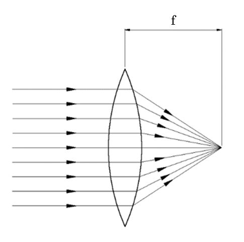
Source: created by the authors.
The characteristics of a negative lens (also called diverging lens) are different from those of its positive counterpart because this type of lenses cause the rays coming from infinity to diverge. Therefore, their focal point cannot be directly observed, as illustrated in Figure 2. In this case, another auxiliary lens should be used to make the rays converge, thus establishing a precise optical criterion to measure the focal length of the diverging lens.
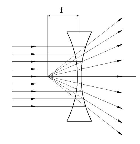
Source: created by the authors.
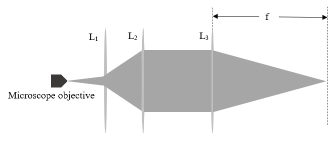
According to geometrical optics, when two thin lenses one positive and one negative are aligned on the optical axis and separated by a d distance, as shown in Figure 3, there is not a single focal length, but rather two: a front focal length (FFL) and a back focal length (BFL), which will be abbreviated as B for the remainder of this paper.
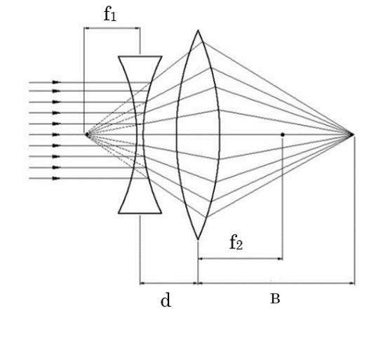
Source: Created by the authors.
To measure B, we know from geometrical optics that it is given by (2):
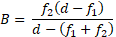 (2)
(2)
Then, from (1), the focal length of the negative lens (f1) is solved in (3) in terms of other variables that can be measured:
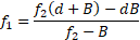 (3)
(3)
2.2 Experimental setup
To guarantee the accuracy of the calibration function, the measurements were made in an area with controlled relative humidity and temperature and positive pressure inside it. The environmental conditions used in this study to conduct the tests are: Temperature 22 °C ± 2 °C and relative humidity (RH) 40 % – 60 %.
The relative humidity and temperature values are optimal for the measurement process because these conditions lie within the acceptable range to measure focal length.
Conversely, if these conditions are not controlled, the measurements of the different focal lengths can be affected because thermal conditions have an impact on material expansion.
To make the measurements, the experimental setup should include a system of thin lenses and a microscope objective on the same axis, as illustrated in Figure. 4. A microscope objective, which is located at the laser output, expands the spot of the beam by making it diverge. Then, the beam hits the L1 negative lens, which increases the divergence of the spot until it reaches a considerable diameter. Then, the L2 positive lens, which is located next, should be positioned with great precision because obtaining a widened spot of constant diameter depends on this step. Once the constant diameter spot has been obtained, it can be considered to have a set of rays coming from infinity. As a result, the focal length of any lens in the L3 position can be accurately measured directly using a previously calibrated tape measure. This setup and this spot are used to find the focal lengths of positive lenses directly.
The microscope objective and lenses L1 and L2 are used to widen the beam
Source: Created by the authors.
To measure the focal length of negative lenses, an auxiliary positive lens is used to converge the rays. In this type of setups, the spot is widened between lenses L2 and L3, but this can be easily verified by placing a screen at least 5 m (infinity) away from L2 and checking if the diameter of the spot remains constant.
Figure. 5 shows the device used for a negative lens such as L3. This setup requires adding an auxiliary positive lens (L4) to achieve the convergence of the rays at a B distance and then indirectly measuring its focal length (f1) using (3) since d, b, and the focal length of L4 are known. In this case, measuring the focal length requires the measurements of the distances of interest involved in (3), which are taken directly using a previously calibrated tape measure.
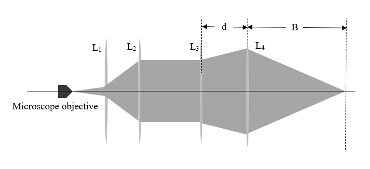
In this case, the L4 positive auxiliary lens is used to converge the beam since L3 is divergent
Source: Created by the authors.
2.3 Mathematical model for determining uncertainty and error in the calibration process of ophthalmic lenses
As established in the measurement method, the assembly was prepared in a laboratory, which facilitated the application of the measurement schemes proposed in Figures 4 and 5 for positive and negative lenses, respectively. Figure 6 shows the assembly, which only requires a rail with lens mounts aligned with the table on which the focal length measurements are made using a calibrated tape measure.
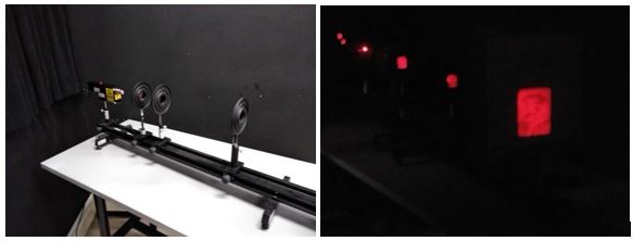
Source: Created by the authors.
The mathematical expression used here to determine the uncertainty is based on stochastic models; therefore, it is based on the Guide for the Expression of Measurement Uncertainty (GUM) [
 (4)
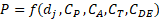
(4)
where f1 is the focal length of the lens; di, the deviation of the measurement at point j, which corresponds to each point taken from the focal length in relation to the reference value; CP, the correction due to the pattern, which corresponds to the tape measure; CA, the correction to compensate for the misalignment effect between the ruler and the table, according to the setup shown in Figure 6; CT, the correction due to differential thermal expansion; and CDE, the correction due to the scale of the tape measure. The deviation of the dj measurement is given by (5):
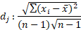 (5)
(5)
where xi is the measurement of each focal length of the lens x ̅, the mean of the measurement of the focal distances of the lens; and n, the number of data obtained. The CP correction is given by (6):
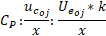 (6)
(6)
where ucoj denotes the product of the expanded uncertainty of the tape measure (Ueoj) multiplied by the 𝑘 coverage factor, which was previously calibrated at a laboratory at Instituto Tecnológico Metropolitano (ITM) in Medellín, Colombia. The CA correction is given by (7):
 (7)
(7)
where θ2max is the correction of the measured angle due to perpendicularity loss, and 𝑥𝑜𝑖 is the measurement of the focal distance of the lens. The CDE correction is given by (8):
 (8)
(8)
where e is the scale being used. In this study, it is millimeters (i.e., 0.001 meter).
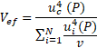
According to the law of propagation of uncertainty, the expression of the combined standard uncertainty, uc2 (P), , for positive lenses (assuming there is no correlation between the variables) is given by (9):
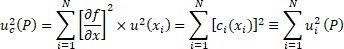 (9)
(9)
Applying the expression above to the function of ophthalmic lens calibration and considering the sources of uncertainty established in (1) and (4), the output variable is given by (10):
 (10)
(10)
Applying (8) in (1) and (3), we obtain (11):
 (11)
(11)
The estimate of the effective degrees of freedom of the standard uncertainty, Uc (P), associated with the output estimate is obtained using the Welch–Satterthwaite formula [4], given by (12):
 (12)
(12)
The k coverage factor can be obtained using this equation, which is derived from a table of values and based on a Student’s t-distribution evaluated for a coverage probability of 95.45 %. A coverage factor of k = 2.0 is used in this study, which must be multiplied by the combined uncertainty, uc, to find the expanded uncertainty, Ue, using (10) and (11) with the result shown in (13).
 (13)
(13)
For negative lenses, we obtain (14):
 (14)
(14)
where f2 is the focal distance of the negative lens, and the uncertainties are the same as those of the positive lens, with one difference, i.e., the term for the auxiliary positive lens, 𝐶𝐿𝑃, which is applied to the same procedures to determine its uncertainty.
According to the law of propagation of uncertainty, the expression of the combined standard uncertainty, uc2 (P), of a negative lens (assuming there is no correlation between the variables) is the same as that presented in (3). Applying the previous step to the ophthalmic lens calibration function and taking into account the sources of uncertainty declared in models (1) and (14), the output variable is given by (15):
 (15)
(15)
Applying (14) in (1) and (9), we obtain Expression (16):
 (16)
(16)
The estimation of the effective degrees of freedom of the standard uncertainty, uc (p), associated with the output estimate is obtained using the previously mentioned Welch–Satterthwaite formula (12). Likewise, a k coverage factor of 2.0 is used here based on a student’s t-distribution for a coverage probability of 95.45 %. These values are taken into account to find the expanded uncertainty in a similar way to the previous case.
3. EXPERIMENTAL RESULTS
The results obtained with the proposed procedure show the estimation of uncertainty in the calibration of ophthalmic lenses in accordance with what is established in a non-stochastic methodology such as the Guide for the Expression of Measurement Uncertainty (GUM) [
The GUM establishes a general structure for evaluating and expressing uncertainty in measurements that can be applied to multiple measurement processes with different levels of accuracy and precision. Moreover, the principles in this guide are intended to be applicable to a wide range of measurements. The steps proposed in the GUM, which were widely used in this paper, are followed to identify and characterize the sources of uncertainty and estimate combined and expanded uncertainties.
To implement the method proposed here and considering that the physical phenomena being intervened are diopter distances, the contributions in document DI-011 [
Source: Created by the authors.
| Lenses | RM | m1 | m2 | m3 | m4 | m5 | m6 | m7 | m8 | m9 | m10 | Aver. | DP |
| l1 | 10.000 | 0.100 | 0.101 | 0.098 | 0.099 | 0.100 | 0.100 | 0.103 | 0.103 | 0.102 | 0.103 | 0.101 | 9.911 |
| l2 | 10.000 | 0.103 | 0.103 | 0.102 | 0.100 | 0.102 | 0.102 | 0.104 | 0.106 | 0.102 | 0.101 | 0.103 | 9.756 |
| l3 | 3.330 | 0.310 | 0.305 | 0.311 | 0.309 | 0.306 | 0.302 | 0.305 | 0.304 | 0.308 | 0.312 | 0.307 | 3.255 |
| l4 | 3.330 | 0.308 | 0.305 | 0.310 | 0.308 | 0.308 | 0.304 | 0.304 | 0.301 | 0.308 | 0.312 | 0.307 | 3.259 |
| l5 | 0.500 | 2.130 | 2.140 | 2.155 | 2.160 | 2.151 | 2.155 | 2.160 | 2.150 | 2.165 | 2.170 | 2.154 | 0.464 |
| l6 | -20.000 | -0.050 | -0.049 | -0.049 | -0.049 | -0.049 | -0.050 | -0.047 | -0.049 | -0.052 | -0.049 | -0.049 | -20.301 |
| l7 | -20.000 | -0.050 | -0.049 | -0.050 | -0.050 | -0.050 | -0.049 | -0.054 | -0.051 | -0.048 | -0.049 | -0.050 | -20.004 |
| l8 | -5.000 | -0.192 | -0.192 | -0.192 | -0.192 | -0.192 | -0.195 | -0.193 | -0.191 | -0.188 | -0.189 | -0.192 | -5.215 |
| l9 | -5.000 | -0.196 | -0.189 | -0.190 | -0.192 | -0.192 | -0.191 | -0.190 | -0.189 | -0.191 | -0.184 | -0.190 | -5.252 |
| l10 | -4.000 | -0.263 | -0.256 | -0.261 | -0.260 | -0.260 | -0.253 | -0.248 | -0.247 | -0.250 | -0.252 | -0.255 | -3.921 |
| lAUX | 10.000 | 0.100 | 0.100 | 0.101 | 0.103 | 0.103 | 0.101 | 0.100 | 0.100 | 0.103 | 0.102 | 0.101 | 9.872 |
Source: Created by the authors.
| Lens | (dj) | Error | Combined uncertainty | Expanded uncertainty |
| l1 | 0.00060 | 0.08900 | 0.00062 | 0.00120 |
| l2 | 0.00055 | 0.24400 | 0.00057 | 0.00110 |
| l3 | 0.00110 | 0.07500 | 0.00112 | 0.00220 |
| l4 | 0.00109 | 0.07100 | 0.00111 | 0.00220 |
| l5 | 0.00392 | 0.03600 | 0.00395 | 0.00790 |
| l6 | 0.00044 | 0.30100 | 0.00046 | 0.00093 |
| l7 | 0.00053 | 0.00400 | 0.00055 | 0.00110 |
| l8 | 0.00069 | 0.21500 | 0.00072 | 0.00140 |
| l9 | 0.00106 | 0.25200 | 0.00108 | 0.00220 |
| l10 | 0.00197 | -0.07900 | 0.00200 | 0.00400 |
| lAUX | 0.00045 | 0.12800 | 0.00047 | 0.00094 |
The uncertainty in the ophthalmic lens calibration function is estimated after obtaining the results in the measurement process, applying (9), (10), (11), (12), (13), (14), and (16) to the data in Table 1. Hence, an error and an expanded uncertainty, 𝑈𝑒, are obtained for each measurement point in Table 2.
Table 1 lists the focal lens measurements with index 1, and subindices in numerical order. In addition, lAUX denotes the auxiliary lens used in the setup for measuring distance B. RM is the reference measurements; DP, dioptric power; and m, the measurement with an index that corresponds to the measurement order.
Table 2 shows the data obtained after applying the mathematical model based on the law of propagation of uncertainty. This law is also used to express the calculation with a type A uncertainty (dj); a type B uncertainty provided by the reference (Cp; the uncertainty due to compensation for the sliding effect between the ruler and the table which is constant with a value of 0.00478 (Ca); the uncertainty due to differential thermal expansion correction and will always taken as zero (Ct); and the uncertainty provided by the scale division of the tape measure which is also taken as zero(Cde). Subsequently, the combined uncertainty is calculated using (16) resulting in a constant value of 0.00041. For the expanded uncertainty, the effective degrees of freedom should be estimated first by applying (12), using a k coverage factor of 2.0 based on a Student’s t-distribution for a coverage probability of 95.45 %. This coverage factor is multiplied by the combined uncertainty so that the expanded uncertainty can be found at each point, as shown in Table 2.
According to the results obtained with the calibration function, a similar behavior can be expected in each repetition of the measurement executed for each nominally true value with the reference diopters, thus obtaining errors of around one diopter, whether for positive or negative lenses. The predominant uncertainty in most points is provided by the calibration of the standard being used (CP). Thus, the other sources that would contribute to the expanded uncertainty are the uncertainty provided by the repeatability (dj) and that provided by the scale division of the tape measure (Cde). This is because the sources due to compensation of the sliding effect between the ruler and the table (Ca), the source due to the differential thermal expansion correction (Ct), and the environmental conditions applied in the laboratory are considered null by the method.
Finally, considering the recommendations provided by the Spanish Metrology Center [
4. CONCLUSIONS
This article presented a procedure for calibrating ophthalmic lenses. Additionally, it proposed a mathematical model for estimating uncertainty based on a non-stochastic methodology such as the Guide for the Expression of Measurement Uncertainty (GUM) [
However, this method may present some limitations compared to existing ones (e.g., the interferometry method) because the measurements are made manually by the operator. In addition, not using a robotic or automated system can lead to human error, and, although this is considered in the estimation of uncertainty, it still is a limitation that would be easily overcome with financial resources. Nevertheless, this study is important because it investigates the reliability of measurements of biomedical equipment, specifically ophthalmic lenses. In addition, it provides relevant information for ophthalmic lens manufacturers because the maximum expanded uncertainty of the method proposed here was optimal: ± 0.0079 diopters in a 0-5 diopters lens. By contrast, other authors [
The focal length measurement procedure used here offers two advantages: simplicity of the assembly and low cost. None of the papers reviewed in this study describes a method based on a cheaper assembly that also presents high stability and easy operation. The current disadvantages of this process are associated with its rudimentary and low-cost implementation that does not use any electronic sensors or measurement components. However, this can be overcome by obtaining financial resources to purchase more accurate measuring instruments.
A future line of research is the application of this calibration function to other ophthalmic equipment based on physical principles to guarantee the validity of the results in order to obtain reliable measurements in eye diagnostics.
5. ACKNOWLEDGMENTS
This study was conducted in the framework of the project developed by Alejandro Salgar-Marin as a young researcher, whose general objective is “To define a calibration method for optical lenses applied to the metrological assurance of ophthalmic instruments.” This study was funded by the Instituto Tecnológico Metropolitano (ITM) in Medellín, Colombia, under the program called “Young researchers and innovators,” which is part of the institutional development plan: “ITM to another level.” The data in this paper were obtained at the physics laboratory and analyzed at the AMYSOD laboratory located in the Parque i research laboratory center at the ITM. Professor Javier Vargas thanks the Faculty of Exact and Applied Sciences, ITM, for their financial support.
CONFLICTS OF INTEREST
The authors declare that there is no conflict of interest.
6. REFERENCES
- arrow_upward [1] O., Tobón; V., Rodríguez, “Desarrollo y estandarización de métodos de calibración para equipos utilizados en salud visual (Queratómetros, Lensómetros y Tonómetros), implementados en el Hospital Universitario de San Vicente Fundación”, RIB, vol. 11, no. 22, pp. 21-28, Oct. 2017. https://doi.org/10.24050/19099762.n22.2017.1179
- arrow_upward [2] Ministerio De Salud Y Protección Social, “Resolución Número 3100 De 2019”. 2019. http://suin-juriscol.gov.co/viewDocument.asp?ruta=Resolucion/30039964
- arrow_upward [3] A. F., Ramirez Barrera, J. F., Martínez Gómez, E., Hidalgo Vásquez, “Modelo de gestión para la aplicación del control metrológico legal y la evaluación de la conformidad en equipos biomédicos”, RIB, vol. 11, no. 21, pp. 73-80, Jun. 2017. https://doi.org/10.24050/19099762.n21.2017.1175
- arrow_upward [4] Joint Committee for Guides in Metrology, “JCGM 100: Evaluation of measurement data – Guide to the expression of uncertainty in measurement”, 2008. https://www.bipm.org/documents/20126/2071204/JCGM_100_2008_E.pdf/cb0ef43f-baa5-11cf-3f85-4dcd86f77bd6
- arrow_upward [5] M. R., de Paiva, O., Pohlmann-Filho, A., Soratto, “Prospection for metrological control in medical scales and sphygmomanometers in the state of Santa Catarina – Brazil”, J. Phys.: Conf. Ser, vol. 575, no. 1, pp. 24-27. Nov. 2013. https://iopscience.iop.org/article/10.1088/1742-6596/575/1/012047
- arrow_upward [6] A. F., Ramírez-Barrera, E., Delgado-Trejos, V., Ramírez-Gómez, “Uncertainty estimation in the sphygmomanometers calibration according to OIML R16-1 from a legal metrology perspective”, IyU, vol. 25, p. 25, Oct. 2021. https://doi.org/10.11144/javeriana.iued25.uesc
- arrow_upward [7] A., Badnjević, L., Gurbeta, D., Bošković, Z., Džemić, “Medical devices in legal metrology”, En 4th Mediterr. Conf. Embed. Comput. MECO, Budva, 2015, pp. 365–367. https://doi.org/10.1109/MECO.2015.7181945
- arrow_upward [8] J. J., Cárdenas-Monsalve, A. F., Ramírez-Barrera, E., Delgado-Trejos, “Evaluación y aplicación de la incertidumbre de medición en la determinación de las emisiones de fuentes fijas: una revisión”, TecnoLógicas, vol. 21, no. 42, pp. 231–244, May. 2018. https://doi.org/10.22430/22565337.790
- arrow_upward [9] J., Zhang, W., Liu, M., Gao, X. Ding, “Metrological calibration of ophthalmometers”, En 8th Int. Conf. Biomed. Eng. Informatics, BMEI, Shenyang, 2015, pp. 360–365. https://doi.org/10.1109/BMEI.2015.7401530
- arrow_upward [10] N. E., Norrby et al., “Accuracy in determining intraocular lens dioptric power assessed by interlaboratory tests.”, J. Cataract Refract. Surg., vol. 22, no. 7, pp. 983–993, Sep. 1996. https://doi.org/10.1016/s0886-3350(96)80204-5
- arrow_upward [11] W., Yang et al., “Research on focal length measurement scheme of self-collimating optical instrument based on double grating”, Sensors, vol. 20, no. 9, May. 2020. https://doi.org/10.3390/s20092718
- arrow_upward [12] R. K., Choudhary, S. M., Hazarika, R. S., Sirohi, “Talbot interferometry for focal length measurement using linear and circular gratings”, Springer Proc. Phys., vol. 194, pp. 639–647, Sep. 2017. https://doi.org/10.1007/978-981-10-3908-9_80
- arrow_upward [13] J. A., Sousa, A. M., Reynolds, Á. S., Ribeiro, “A comparison in the evaluation of measurement uncertainty in analytical chemistry testing between the use of quality control data and a regression analysis”, Accredit. Qual. Assur., vol. 17, no. 2, pp. 207–214, Jan. 2012. https://doi.org/10.1007/s00769-011-0874-y
- arrow_upward [14] Y., Nakano, K., Murata, “Talbot interferometry for measuring the focal length of a lens”, Appl. Opt., vol. 24, no. 19, pp. 3162-3166, Oct. 1985. https://doi.org/10.1364/AO.24.003162
- arrow_upward [15] P., Singh, M. S., Faridi, C., Shakher, R. S., Sirohi, “Measurement of focal length with phase-shifting Talbot interferometry”, Appl. Opt., vol. 44, no. 9, pp. 1572–1576, Mar. 2005. https://doi.org/10.1364/AO.44.001572
- arrow_upward [16] L. M., Bernardo, O. D. D., Soares, “Evaluation of the focal distance of a lens by Talbot interferometry”, Appl. Opt., vol. 27, no. 2, pp. 296-301, Jan. 1988. https://doi.org/10.1364/AO.27.000296
- arrow_upward [17] K. V., Sriram, M. P., Kothiyal, R. S., Sirohi, “Direct determination of focal length by using Talbot interferometry”, Appl. Opt., vol. 31, no. 28, pp. 5984-5987, Oct. 1992. https://doi.org/10.1364/AO.31.005984
- arrow_upward [18] G., Yang, L., Miao, X., Zhang, C., Sun, Y., Qiao. “High-accuracy measurement of the focal length and distortion of optical systems based on interferometry”, Appl Opt., vol. 57, no. 18, pp. 5217-5223, Jun. 2018. https://doi.org/10.1364/AO.57.005217
- arrow_upward [19] I., Glatt, O., Kafri, “Determination of the focal length of nonparaxial lenses by moire deflectometry”, Appl. Opt., vol. 26, no. 13, pp. 2507-2508, Jul. 1987. https://doi.org/10.1364/AO.26.002507
- arrow_upward [20] S., Trivedi, J., Dhanotia, S., Prakash, “Measurement of focal length using phase shifted moiré deflectometry”, Opt. Lasers Eng., vol. 51, no. 6, pp. 776–782, Jun. 2013. https://doi.org/10.1016/j.optlaseng.2013.01.018
- arrow_upward [21] E., Keren, K. M., Kreske, O., Kafri, “Universal method for determining the focal length of optical systems by moire deflectometry”, Appl. Opt., vol. 27, no. 8, pp. 1383-1385, Apr. 1988. https://doi.org/10.1364/AO.27.001383
- arrow_upward [22] S., De Nicola, P., Ferraro, A., Finizio, G., Pierattini, “Reflective grating interferometer for measuring the focal length of a lens by digital moiré effect”, Opt. Commun., vol. 132, no. 5–6, pp. 432–436, Dec. 1996. https://doi.org/10.1016/0030-4018(96)00391-4
- arrow_upward [23] Y. P., Kumar, S. ,Chatterjee, “Technique for the focal-length measurement of positive lenses using Fizeau interferometry”, Appl. Opt., vol. 48, no. 4, pp. 730–736, Jan. 2009. https://doi.org/10.1364/AO.48.000730
- arrow_upward [24] L., Angel, M., Tebaldi, R., Henao, “Phase stepping in Lau interferometry”, Opt. Commun., vol. 164, no. 4-6, pp. 247–255, Jun. 1999. https://doi.org/10.1016/S0030-4018(99)00172-8
- arrow_upward [25] M., Thakur, C., Shakher, “Evaluation of the focal distance of lenses by white-light Lau phase interferometry”, Appl. Opt., vol. 41, no. 10, pp. 1841-1845, Apr. 2002. https://doi.org/10.1364/AO.41.001841
- arrow_upward [26] M., de Angelis, S., De Nicola, P., Ferraro, A., Finizio, G. Pierattini, “A new approach to high accuracy measurement of the focal lengths of lenses using a digital Fourier transform”, Opt. Commun., vol. 136, no. 5–6, pp. 370–374, Apr. 1997. https://doi.org/10.1016/S0030-4018(96)00730-4
- arrow_upward [27] L., Chen, J., Hong, Y., Qiao, X., Zheng, X., Sun, “Theoretical analysis of collimators on the geometrical calibration of wide field-of-view radiometer”, Optik, vol. 121, no. 3, pp. 302–305, Feb. 2010. https://doi.org/10.1016/j.ijleo.2008.02.028
- arrow_upward [28] S., De Nicola, P., Ferraro, A., Finizio, G., Pierattini, “Reflective grating interferometer for measuring the focal length of a lens by digital moire effect”, Opt. Commun., vol. 132, no. 5–6, pp. 432–436, 1996. https://doi.org/10.1016/0030-4018(96)00391-4
- arrow_upward [29] D., Fantanas, A., Brunton, S. J., Henley, R. A., Dorey, “Investigation of the mechanism for current induced network failure for spray deposited silver nanowires”, Nanotechnology, vol. 29, no. 46, p. 465705. Sep. 2018. https://doi.org/10.1088/1361-6528/aadeda
- arrow_upward [30] E. H. K., Stelzer, S., Grill, “The uncertainty principle applied to estimate focal spot dimensions”, Opt. Commun., vol. 132, no. 1–6, pp. 51-56, Jan. 2000. https://doi.org/10.1016/S0030-4018(99)00644-6
- arrow_upward [31] M., Dashtdar, S., Ali Hosseini-Saber, “Focal length measurement based on Fresnel diffraction from a phase plate”, Appl. Opt., vol. 55, no. 26, p. 7434-7437, Sep. 2016. https://doi.org/10.1364/AO.55.007434
- arrow_upward [32] M., Azpurua, C., Tremola, E. J., Paez, “Comparison of the GUM and Monte Carlo Methods for the Uncertainty Estimation In Electromagnetic Compatibility Testing”, Prog. Electromagn. Res. B, vol. 34, pp. 125-144, 2011. http://www.jpier.org/PIERB/pier.php?paper=11081804
- arrow_upward [33] O., Sima, M. C., Lépy, “Application of GUM Supplement 1 to uncertainty of Monte Carlo computed efficiency in gamma-ray spectrometry”, J. apradiso., vol. 109, pp. 493-499, Mar. 2016. https://doi.org/10.1016/j.apradiso.2015.11.097
- arrow_upward [34] Centro Español de Metrología “Procedimiento DI-011 para la calibración de flexómetros”, 2021.