Received: March 18, 2022
Accepted: August 17, 2022
Available: November 2, 2022

 

 

---

Abstract

This research focused on the development of a methodology for calculating the optimal power factor (OPF) in microgrids with the photovoltaic generation, in order to use solar inverters as reactive compensators, which will change their power factor according to the needs of the load. The developed methodology proposes a convex optimization model with multiple constraints to solve the OPF problem. Wirtinger's linearization in the power balance equation was implemented. The stochastic behavior of solar radiation was considered using the average sampling approach (ASA) to generate solar scenarios, which are used to calculate the magnitude of the generation of photovoltaic systems for specific hours of the day. Finally, the algorithm was run on CIGRE's 19-node test grid. The proposed methodology showed that as the radiation level increases during the day, more radiation scenarios can be tested, which increases the accuracy of the power factor value for each PV system. Although the general idea in power systems is to have a unity power factor, the algorithm resulted in power factors with values less than one in some inverters. This represents an injection of reactive power from the inverters to meet the reactive needs of the loads connected close to said PV generators, which is reflected in a variation in the magnitude of the power factor.

Resumen

Esta investigación se centró en el desarrollo de una metodología para el cálculo del factor de potencia óptimo (OPF) en micro redes con generación fotovoltaica, con el fin de usar los inversores solares como compensadores reactivos, los cuales cambiaran su factor de potencia de acuerdo a las necesidades de la carga. La metodología desarrollada planteó un modelo de optimización convexo con múltiples restricciones para resolver el problema de OPF; además, fue implementada la linealización de Wirtinger en la ecuación de balance de potencia. Se consideró el comportamiento estocástico de la radiación solar utilizando la aproximación de muestreo promedio (ASA) para generar escenarios solares, los cuales son usados para calcular la magnitud de la generación de los sistemas fotovoltaicos para horas específicas del día. Finalmente, se ejecutó el algoritmo en la red de pruebas de 19 nodos de CIGRE. La metodología propuesta mostró que, a medida que el nivel de radiación incrementa en el transcurso del día, más escenarios de radiación pueden ser puestos a prueba, lo cual aumenta la precisión del valor de factor de potencia para cada sistema PV. Aunque la idea general en los sistemas de potencia es tener un factor de potencia unitario, el algoritmo brindó como resultado factores de potencia con valores inferiores a uno en algunos inversores. Esto representa una inyección de potencia reactiva desde los inversores para suplir las necesidades de reactivos de las cargas conectadas cerca a dichos generadores PV, lo cual se refleja en una variación en la magnitud del factor de potencia.

NOMENCLATURE

---

1. INTRODUCTION

---

Modern distribution systems are characterized by high penetration of renewable energies such as wind and photovoltaics, which are integrated into the network through power inverter devices. Overcrowding in the installation of these devices has led to overvoltage, power factor violation, voltage imbalance, and other issues in electrical networks. Therefore, it is necessary to develop a methodology that allows for efficient control of the reactive power resources of these devices [1]. Like FACT devices, inverters are built based on power electronics, and they have advantages such as high conversion efficiency, improved power quality, active and reactive power control, among others [2]-[4]. Although these converters have some power factor compensation capabilities, they are usually operated at a unit power factor. This operation mode reduces the efficiency of the entire system [5]. One of the most promising ways to solve this problem is by including communications and a power factor management system. However, this approach is still expensive in many practical applications. Therefore, an optimization model for the power factor is required in order to define a fixed set point while considering the stochastic behavior of solar generation. This paper presents a methodology for defining this fixed set point, based on a series of convex approximations. Three-phase modeling of the grid is proposed, considering single and three-phase converters. The physical limitations of the converters are also considered, and the grid equations are linearized by using Wirtinger's calculus. The sample average approximation considers the stochastic behavior of solar radiation to maintain the problem convex and computationally tractable. Real data for solar radiation is considered and applied to the CIGRE benchmark [6], [7].

Several methods have been proposed before to solve this problem. In [8], a decentralized self-adjusting reactive power controller was presented, whose objective was to compensate for the reactive power of local loads and share the reactive power of non-local loads. That control included a drop constant that was adjusted according to the reactive power. Hatziargyriou et al. [9] considered using a generalized DC power flow and quadratic programming in order to obtain an optimal reactive power flow to control the reactive power supplied by each distributed generator. In [10] was proposed a wireless control strategy using optimized virtual impedance controllers and load measurements of reactive power-sharing throughout the network. A genetic algorithm was used to define each distributed generator's virtual impedance parameters, which reduce the global reactive power-sharing error. In [11] was presented the concept of stochastic game modeling from game theory to develop an algorithm with the purpose of solving a multi-objective optimization, which included the reactive power reserve maximization and the improvement of the voltage profile. Wang et al. [12] showed a control strategy for islanded microgrids which used small-signal models, state estimators, optimal regulators, and optimal control. All these allowed for voltage regulation without communication systems. In [13] was presented a review of multiple sharing strategies of active and reactive power in hierarchically controlled microgrids. Morais et al. [14] mentioned multiple reactive power control strategies considering the smart grid paradigm, the management of distributed energy resources, and a distributed network aggregator, namely a Virtual Power Plant, which was proposed and implemented in a simulation tool. In [15] was proposed a bibliographical review of mathematical methods used for optimal selection and location of reactive power compensating elements applied to distribution systems, most of them based on metaheuristics. Few articles study the stochasticity of renewable resources and their load on microgrids. Some, like [16] and [17], carry out their investigation by performing a mathematical analysis of all the components and stochastic behavior of the system in order to obtain an optimal power flow and reduce losses.

In [18], a stochastic multi-objective optimal dispatch was applied to grids with wind farms. This is in order to solve the problem of voltage stability and reactive power reserve (RPR) by minimizing the payments of energy and maximizing the RPR under wind power generation uncertainty using a combination of the lexicographic optimization technique and the augmented-weighted ∈ -constraint method. Nazmul et al. [19] presented a review of reactive power management strategies and optimization algorithms applied to power electronic converters for renewable energy generators in order to solve steady-state voltage and dynamic stability issues. In [20] were presented two methodologies to use the reactive power capabilities of smart inverters on photovoltaic installations: the first one limits the amount of active power, which implies a reduction of PV production; and the second one oversize the inverter, which allows for better reactive power reserves.

In [21], mixed integer linear programming linked with two stochastic stages is used to study the resilience of a microgrid under extreme conditions while considering reactive power management. Abreu et al. [22] used stochastic optimal power flow to optimize the use of reactive power. This technique allows selecting the distributed energy resource that can provide reactive power by limiting the reactive power supplied by the transmission system operator, thus reducing losses. In [23] was developed a reactive power methodology considering photovoltaic inverter capabilities and fixed capacitors. A mixed integer second-order conic programming model is used, minimizing the maintenance and operation cost of compensation devices, thus confirming a considerable reduction in investment and energy losses in distribution grids.

Mehbodniya et al. [24] mentioned the effects of renewable energy (e.g., wind and photovoltaic) on distribution grids. The objective function of the model minimizes the operating cost of the system, and stochastic programming is used to solve the formulated linear problem by improving the active and reactive power losses, the network energy cost, and the voltage deviation by more than 30 %.

As mentioned earlier, the main differences between the approaches are as follows. i) The proposed model is convexified by using Wirtinger linearization on the power flow equations [25]. This linearization allows guaranteeing the global optimum in the approximated model with a high accuracy and fast convergence of the interior point algorithms. ii) The proposed model considers the stochastic behavior of solar generation directly by using sample average approximation. This approximation considers the stochastic nature of solar radiation and the loads without jeopardizing the convergence and uniqueness properties of the convex model. iii) The implementation of the proposed methodology can be executed directly in commercial converters, as it does not require communications or real-time operation. This, with the main purpose of scheduling the power factor of the converter for each type of day and each hour without a master controller.

The rest of the article is organized as follows. Section 2 presents the problem statement, where the objective function and the constraints are presented while considering the conventional non-linear non-convex representation of the grid, the convex formulation, and the relaxation of the power flow equation using Wirtinger linearization. The stochastic model is also explained. Finally, the grid model and algorithm simulation results of each test case are presented in Section 3, followed by the conclusions, acknowledgments, and relevant references. This article is part of a selection of the best works presented at the Symposium X SICEL -2021.

2. MATERIALS AND METHODS

---

2.1 Model Definition

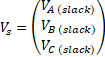
Let us consider a microgrid represented by the three-phase nodal admittance matrix , which is divided in two sub-matrices, namely Y_S for the substation and Y_N for the rest of the nodes. A three-phase representation of the grid is considered, so the slack node has three components, as given in (1):

Model 1. Complete model for the optimal set point of the reactive power in a three-phase grid.

The grid is therefore represented by the following non-linear/non-affine model (2):

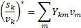
Where * represents the complex conjugate operator, and v_k, v_m ∈ V_N, y_km ∈ Y_N. The optimization model consists of minimizing the expected value of the total losses p_L, which is subject to technical constrains as follows (3)-(7):

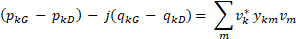
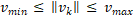
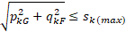
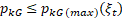
Where (3) is a convex function that represents the expected losses of the network, (4) are non-linear and non-convex equations that represent the active and reactive power flow constraints, respectively, (5) is the maximum and minimum voltage of the grid, (6) is the capability of the converter, and (7) is the maximum power that can be generated in each node.

Note that (6) depends on the converter, whereas (7) depends on the primary resource (i.e., the scenario of the irradiance ξ_t). Therefore, P_kG(max) is a random variable. It is important to note that (4) is maintained in complex form for the sake of a simple representation. However, this equation needs to be separated into real and imaginary parts.

This problem is difficult to solve due to the non-linear non-convex nature of the power flow equations and the stochastic nature of the model. In the next section, the model is simplified for a deterministic case in order to obtain a convex model (see [26] for a formal definition of convexity). After that, in section 2.4, the stochastic model is considered.

2.2 Convex Formulation

The problem of non-convexity and non-linearity mentioned in Subsection 2.2 must be relaxed to obtain a tractable model. There are different linearizations proposed in the literature, where the ones presented by [27]-[29] stand out.

Although each of these linearizations comes from a different theoretical background, they are equivalent for values close to 1 p.u. In this paper, a linearization based on Wirtinger's calculus is used. Like the previous linearization, this is equivalent to values close to 1 p.u. However, the advantage of this approach is that it guarantees an affine separation between voltages and powers in the optimization model. The distributed resources are considered by using a ZIP model. A deep mathematical analysis of this linearization is beyond the objectives of this paper but can be found in [25]. The approximated representation of a three-phase grid-connected is given by (8):

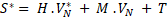
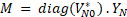
Where H, M, T are constant matrices defined by (9)-(11):

Therefore, constraint (4) can be represented as follows (12):

Note that (12) defines an affine space, even when it is separated into real and imaginary parts, since neither H, M or Tdepends on the power.

2.3 Stochastic Model

The proposed model is designed for microgrids and small power distribution systems. Therefore, the irradiance scenario is the same for all the panels in the grid. The methodology takes real data for generated power and defines η_t scenarios with probability ξ_t. In this situation, the expected value of the losses can be represented by the following sample average approximation (ASA), which defines an affine (13):

Where ξ_t is the probability of each scenario –the number of scenarios can grow very fast in many power systems applications. However, the main supposition of this work is that the solar panels are very close geographically, and hence the scenario is the same in all the panels along the microgrid. In this situation, the value of ηt is small, as it will be presented in the results. Collecting all the aforementioned approximations, the model takes the following structure (14) - (15) and the (5)- (7):

Model 2. Approximated convex model for the optimal power factor in a three-phase grid.

Note that this model is convex and tractable if the number of scenarios is finite. The power factor can be calculated after the optimization model is solved by using the values of p and q. In the next section, the generation of these scenarios will be presented.

3. RESULTS AND DISCUSSION

---

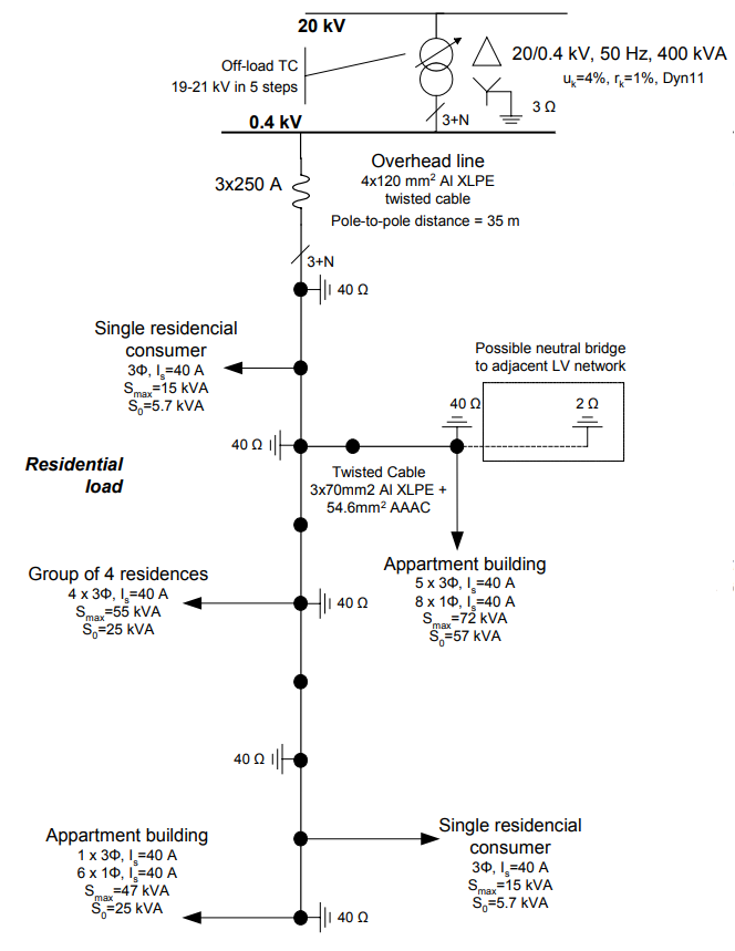
The proposed model was evaluated on the CIGRE benchmark [6] (see Figure 1). The stochastic phenomenon was modeled as a set of scenarios using a database of irradiance with 8605 values taken at Universidad Tecnológica de Pereira (UTP). The information was collected using a device developed by UTP students. This device saved irradiance information in 5-minute intervals during September 2012. Using this database, five values with different solar radiation magnitudes were generated. These scenarios were obtained by grouping the solar radiation values through Matlab’s histogram (his) function.

Here, the his.Values function represents the frequency of occurrence of each value, and the his.binedges function represents the radiation value associated with the frequency. This allows to better differentiate the results, as a general radiation value is not used for the entire operating time of the photovoltaic installation; these radiation levels change hour by hour, which implies greater precision in the results. This process is applied for three cases: one at sunrise (6:00 a.m.), another one at mid-morning (9:00 a.m.), and the last one at the maximum solar radiation point (12:00 p.m.). Figure 2 shows the number of scenarios and their corresponding frequency (which can be transformed into probability).

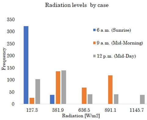
As shown in Figure 2, the radiation level is different in every case, at sunrise, a high frequency of occurrence on low radiation values (127.3 W/m²) and low frequency on high radiation levels can be observed.

This means that, at 6:00 a.m., the radiation received is low and, over the course of the hours, the frequency of occurrence in the other radiation values increases (mid-morning, mid-day), which represents an increase in the radiation received by the photovoltaic installation. With that in mind, the generation of the system is going to change in any case, thus allowing to obtain different power factor profiles for each scenario.

Equation (14) presents a minimization of the losses, optimizing the active and reactive power supplied by each solar power plant connected to the microgrid.

Starting from the basic definition of power factor (16) – (18), p element on (19) is defined, which limits the amount of reactive power in the grid. This is obtained as a result of the convex model programmed on MATLAB. Hence, the power factor for each optimized solar source can be obtained.

Our test system is based on CIGRE microgrid, which uses the same conductor type and grid scheme, albeit with some modifications. This microgrid has three mono-phase generators connected to each phase of node 2, three-phase solar generators connected to nodes 7, 13, and 18, with six unbalanced loads located at nodes 3, 8, 11, 14, and 15. The model was solved using the CVX convex optimization library for MATLAB, which was developed by Stanford University and executed on a computer with an Intel i7 processor and 6 GB of RAM.

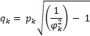
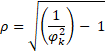
3.1 Case 1 – 6:00 a.m.

This case was evaluated at 6:00 a.m. with a computational time of 11.0507 seconds. Here, the radiation level is low, and, as shown in Figure 2, the amount of data can only represent the first two of the five radiation scenarios. In Figure 3, graphs (a) and (b) plot the possible power factors for generation units 1 and 3 as an outcome of the optimization algorithm. The number of power factors presented on the graphic is related to the level of radiation and the frequency of occurrence obtained at sunrise (two scenarios: 127.3 W/m² and 381.9 W/m²). Table 1 presents the result of (13), which represents the sum of the power factors by their frequency of occurrence, which yields the result of the expected value of the PF for each solar generation inverter unit. This value will be adjusted in the inverters to ensure an efficient operation of the network at that hour of the day. Most of the PV generation nodes were set to one, except on node 13, in which the power factor is lower than one. This represents a reactive power current flowing from the PV inverters to the grid to supply the needs of reactive power near the node 13.

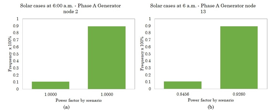
3.2 Case 2 – 9:00 a.m.

The second test was evaluated at 9:00 a.m. with a computational time of 12.13337 seconds. In this case, the radiation level is higher than case 1, and, as shown in Figure 2, the amount of data can represent four out of five scenarios. In Figure 4, graphs (a) and (b) plot the possible power factors for generation units 1 and 3 as an outcome of the optimization algorithm. The number of power factors presented in the graph are related to the level of radiation and the frequency of occurrence obtained at mid-morning (four scenarios: 127.3 W/m², 381.9 W/m², 636.5 W/m², and 891.1 W/m²). Table 2 presents the result of (13), which represents the sum of the power factors by their frequency of occurrence, thus yielding the result of the expected value of the PF for each solar generation inverter unit.

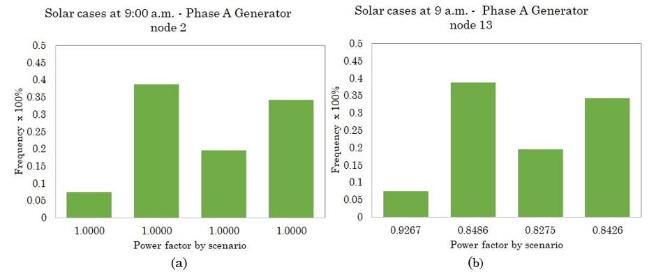
This value will be adjusted in the inverters to ensure an efficient operation of the network at that hour of the day. It can be observed that, for this case, two PV sources located on nodes 7 and 13 set their power factor to a value lower than one, which is due to an increase in the reactive power needs of the loads located near said nodes, which are supplied by the inverters of the sources.

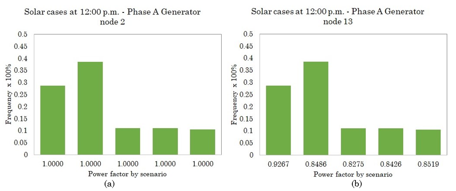
3.3 Case 3 – 12:00 m.

This case was evaluated at 12:00 p.m. with a computational time of 11.5454 seconds. In this case, the radiation level is higher than in cases 1 and 2. As shown in Figure 2, the amount of data was enough to fit all the five proposed scenarios. In Figure 5, graphs (a) and (b) plot the possible power factors for generation units 1 and 3 as an outcome of the optimization algorithm. The number of power factors presented in the graph are related to the level of radiation and the frequency of occurrence obtained at midday (five scenarios: 127.3 W/m², 381.9 W/m², 636.5 W/m², 891.1 W/m², and 1145.7 W/m²). Table 3 presents the result of (13), which represents the sum of the power factors by their frequency of occurrence, thus yielding the result of the expected value of the PF for each solar generation inverter unit. This value will be adjusted in the inverters to ensure an efficient operation of the network at that hour of the day. As in the previous case, the sources connected to nodes 7 and 13 reduce their power factor because of more oversized loads and due to the fact that they are connected near said generation nodes, so their PF is altered since it must supply the necessary reactive power to feed the load.

4. CONCLUSIONS

---

The development of an alternative methodology for reactive power management in microgrids was presented in this document. This methodology allows using linearized models, stochastic analysis, and convex optimization, the use of the capability of PV inverters to be programmed with a set of multiple power factor values which will change throughout the day. Traditionally, the main idea in power systems is to have a unitary power factor, which represents a completely resistive load. However, in the real world, there is no completely resistive load due to the multiple devices that inject or consume reactive power.

With this in mind, it was found that, in small microgrids with a high inclusion of photovoltaic generation, as the magnitude of the radiation increases during the day, photovoltaic sources increase their active power, but the power inverters tend to decrease their power factor to values lower than a unitary power factor. This implies an injection of reactive power from the sources to the grid to supply the load needs, which change over time. This injection of reactive power helps to reduce losses, increase the power transmission of the grid, and improve the voltage profiles.

An optimal setting of the power factor in multiple power inverters may replace the function of some capacitor banks or other reactive compensation devices in a microgrid. Moreover, our methodology allows to effectively set the power factor behavior of the sources with previous study of the grid and load for hourly operation throughout the day and year without the need for a master controller or communication devices that could increase the cost of the microgrid, making the small-scale use of these technologies viable.

5. ACKNOWLEDGMENTS AND FUNDING

---

We would like to thank the research groups, and Electrical and Computing Engineering faculties of Universidad Nacional Autónoma de Mexico, Universidad Distrital Francisco José de Caldas, and Universidad Tecnológica de Pereira. The Project did not receive funding from any public or private institution.

CONFLICTS OF INTEREST

---

The authors declare no financial, professional, or personal conflict of interest arising from the publication of this article.

AUTHOR CONTRIBUTIONS

---

Alexander Casilimas: Design and programming of mathematical algorithms and stochastic analysis.

Óscar Danilo Montoya: Test case development, edition of concepts and contents of the article.

Alejandro Garcés: Operative information of MATLAB CVX library and establishment of the methodology.

César Angeles Camacho: Review and editing of the different chapters of the document, theory, and recommendations on the development methodology.

6. REFERENCES

---

• arrow_upward [1]   W. Y. Atmaja, M. P. Lesnanto, and E. Y. Pramono, “Hosting Capacity Improvement Using Reactive Power Control Strategy of Rooftop PV Inverters,” In 2019 IEEE 7th International Conference on Smart Energy Grid Engineering (SEGE), Oshawa, Canada: SEGE, Aug. 2019, pp. 213-217. IEEE, https://doi.org/10.1109/SEGE.2019.8859888
• arrow_upward [2]   M. Rabiul-Islam, A. M. Mahfuz-Ur-Rahman, K. M. Muttaqi, and D. Sutanto, “State-of-The-Art of the Medium-Voltage Power Converter Technologies for Grid Integration of Solar Photovoltaic Power Plants,” IEEE Transactions on Energy Conversion, vol. 34, no. 1, pp. 372–384, Mar. 2019, https://doi.org/10.1109/TEC.2018.2878885
• arrow_upward [3]   S. Amara and H. Abdallah-Hsan, "Power system stability improvement by FACTS devices: A comparison between STATCOM, SSSC and UPFC," in 2012 First International Conference on Renewable Energies and Vehicular Technology, Nabeul, Tunisia: March 2012, pp. 360-365, https://doi.org/10.1109/REVET.2012.6195297
• arrow_upward [4]   C. Ángeles-Camacho, and F. Bañuelos-Ruedas, "FACTS: Its Role in the Connection of Wind Power to Power Networks", in Wind Farm - Impact in Power System and Alternatives to Improve the Integration. London, United Kingdom: IntechOpen, 2011, pp. 93-108. https://doi.org/10.5772/21200
• arrow_upward [5]   W. Lu, S. Lang, L. Zhou, H. H. C. Iu, and T. Fernando, “Improvement of stability and power factor in PCM controlled boost PFC converter with hybrid dynamic compensation,” IEEE Transactions on Circuits and Systems I: Regular Papers, vol. 62, no. 1, pp. 320–328, Jan. 2015, https://doi.org/10.1109/TCSI.2014.2346111
• arrow_upward [6]   N. Hatziargyriou, S. Papathanassiou, S. Papathanassiou, N. Hatziargyriou, and K. Strunz, “A benchmark low voltage microgrid network.” in Proceedings of the CIGRE symposium: power systems with dispersed generation, Athens, 01 2005, pp. 1-8. https://www.researchgate.net/profile/.pdf
• arrow_upward [7]   A. Garcés, W. Gil-González, O. D. Montoya, H. R. Chamorro, and L. Alvarado-Barrios, “A Mixed-Integer Quadratic Formulation of the Phase-Balancing Problem in Residential Microgrids,” Applied Sciences, vol. 11, no. 5, pp. 1972, Feb. 2021, https://doi.org/10.3390/app11051972
• arrow_upward [8]   M. Hamzeh, H. Mokhtari, and H. Karimi, “A decentralized self-adjusting control strategy for reactive power management in an islanded multi-bus MV microgrid,” Canadian Journal of Electrical and Computer Engineering, vol. 36, no. 1, pp. 18–25, 2013, https://doi.org/10.1109/CJECE.2013.6544468
• arrow_upward [9]   S. Bolognani and S. Zampieri, “A distributed control strategy for reactive power compensation in smart microgrids,” IEEE Transactions on Automatic Control, vol. 58, no. 11, pp. 2818–2833, 2013, https://doi.org/10.1109/TAC.2013.2270317
• arrow_upward [10] Y. Zhu, F. Zhuo, F. Wang, B. Liu, R. Gou, and Y. Zhao, “A virtual impedance optimization method for reactive power sharing in networked microgrid,” IEEE Transactions on Power Electronics, vol. 31, no. 4, pp. 2890–2904, Apr. 2016, https://doi.org/10.1109/TPEL.2015.2450360
• arrow_upward [11] M. A. Arif, M. Ndoye, G. V. Murphy, and K. Aganah, “A stochastic game framework for reactive power reserve optimization and voltage profile improvement,” in 2017 19th International Conference on Intelligent System Application to Power Systems (ISAP), San Antonio TX, Sep. 2017, pp. 1–6. https://doi.org/10.1109/ISAP.2017.8071372
• arrow_upward [12] Y. Wang, X. Wang, Z. Chen, and F. Blaabjerg, “Distributed optimal control of reactive power and voltage in islanded microgrids,” in Conference Proceedings - IEEE Applied Power Electronics Conference and Exposition - APEC, May 2016, vol. 2016-May, pp. 3431–3438. https://doi.org/10.1109/APEC.2016.7468360
• arrow_upward [13] Y. Han, H. Li, P. Shen, E. A. A. Coelho, and J. M. Guerrero, “Review of Active and Reactive Power Sharing Strategies in Hierarchical Controlled Microgrids,” IEEE Transactions on Power Electronics, vol. 32, no. 3, pp. 2427–2451, Mar. 01, 2017. https://doi.org/10.1109/TPEL.2016.2569597
• arrow_upward [14] H. Morais, T. Sousa, P. Faria and Z. Vale, "Reactive power management strategies in future smart grids," in 2013 IEEE Power & Energy Society General Meeting, 2013, pp. 1-5. https://doi.org/10.1109/PESMG.2013.6672332
• arrow_upward [15] A. Águila-Téllez, G. L. Opez, I. Isaac, and J. W. Gonz Alez, “Optimal reactive power compensation in electrical distribution systems with distributed resources. Review,” Heliyon, 2018, vol. 4, p. 746. https://doi.org/10.1016/j.heliyon.2018.e00746
• arrow_upward [16] V. Kekatos, G. Wang, A. J. Conejo, and G. B. Giannakis, “Stochastic Reactive Power Management in Microgrids with Renewables,” IEEE Transactions on Power Systems, vol. 30, no. 6, pp. 3386–3395, Nov. 2015, https://doi.org/10.1109/TPWRS.2014.2369452
• arrow_upward [17] S. M. Mohseni‐Bonab and A. Rabiee, “Optimal reactive power dispatch: a review, and a new stochastic voltage stability constrained multi‐objective model at the presence of uncertain wind power generation”. IET Generation, Transmission & Distribution, vol. 11, no. 4, pp. 815-829, March 2017. https://doi.org/10.1049/iet-gtd.2016.1545
• arrow_upward [18] M. Ghaljehei, Z. Soltani, J. Lin, G. B. Gharehpetian, and M. A. Golkar, “Stochastic multi-objective optimal energy and reactive power dispatch considering cost, loading margin and coordinated reactive power reserve management,” Electric Power Systems Research, vol. 166, pp. 163–177, Jan. 2019, https://doi.org/10.1016/J.EPSR.2018.10.009
• arrow_upward [19] M. Nazmul, I. Sarkar, G. Meegahapola, M. Datta, and L. G. Meegahapola, “Reactive Power Management in Renewable Rich Power Grids: A Review of Grid-Codes, Renewable Generators, Support Devices, Control Strategies and Optimization Algorithms,” IEEE Access, vol. 6, pp. 41458-41489, Aug. 2018, https://doi.org/10.1109/ACCESS.2018.2838563
• arrow_upward [20] J. F. Gómez-González et al., “Reactive power management in photovoltaic installations connected to low-voltage grids to avoid active power curtailment,” Renewable Energy and Power Quality Journal, vol. 1, no. 16, pp. 5–11, Apr. 2018, https://doi.org/10.24084/repqj16.003
• arrow_upward [21] A. Shaker, A. Safari, and M. Shahidehpour, “Reactive Power Management for Networked Microgrid Resilience in Extreme Conditions,” IEEE Transactions on Smart Grid, vol. 12, no. 5, pp. 3940–3953, Sept. 2021, https://doi.org/10.1109/TSG.2021.3068049
• arrow_upward [22] T. Abreu, T. Soares, L. Carvalho, H. Morais, T. Simão, and M. Louro, “Reactive Power Management Considering Stochastic Optimization under the Portuguese Reactive Power Policy Applied to DER in Distribution Networks,” Energies, vol. 12, no. 21, p. 4028, Oct. 2019, https://doi.org/10.3390/en12214028
• arrow_upward [23] S. Souri, H. M. Shourkaei, S. Soleymani, and B. Mozafari, “Flexible reactive power management using PV inverter overrating capabilities and fixed capacitor,” Electric Power Systems Research, vol. 209, p. 107927, Aug. 2022, http://doi.org/10.1016/J.EPSR.2022.107927
• arrow_upward [24] A. Mehbodniya, A. Paeizi, M. Rezaie, M. Azimian, H. Masrur, and T. Senjyu, “Active and Reactive Power Management in the Smart Distribution Network Enriched with Wind Turbines and Photovoltaic Systems,” Sustainability, vol. 14, no. 7, p. 4273, April2022, https://doi.org/10.3390/su14074273
• arrow_upward [25] D. A. Ramírez, A. Garcés, and J. Mora-Florez, "A Wirtinger Linearization for the Power Flow in Microgrids," in 2019 IEEE Power & Energy Society General Meeting (PESGM), Atlanta, 2019, pp. 1-5, https://doi.org/10.1109/PESGM40551.2019.8973647
• arrow_upward [26] S. P. Boyd and L. Vandenberghe, Convex optimization. 1st ed., Cambridge University Press, 2004. https://doi.org/10.1017/CBO9780511804441
• arrow_upward [27] S. Bolognani and S. Zampieri, “On the existence and linear approximation of the power flow solution in power distribution networks,” IEEE Transactions on Power Systems, vol. 31, no. 1, pp. 163–172, Jan. 2016, https://doi.org/10.1109/TPWRS.2015.2395452
• arrow_upward [28] J. R. Martí, H. Ahmadi, and L. Bashualdo, “Linear power-flow formulation based on a voltage-dependent load model,” IEEE Transactions on Power Delivery, vol. 28, no. 3, pp. 1682–1690, 2013, https://doi.org/10.1109/TPWRD.2013.2247068
• arrow_upward [29] Y. Wang, N. Zhang, H. Li, J. Yang, and C. Kang, “Linear three-phase power flow for unbalanced active distribution networks with PV nodes”. CSEE Journal of Power and Energy Systems, vol. 3, no. 3, pp. 321-324, Sept. 2017, https://doi.org/10.17775/CSEEJPES.2017.00240